It seemed like a normal Friday until mid-afternoon. But on 4 February 2022, I embarked on a journey that, at the time, seemed to stretch impossibly far into the future — a future that wasn’t entirely known yet. In the APL Orchard chat room on Stack Exchange, a dozen APLers, some experts and some newbies, held the very first APL Quest chat event.
In this first session, we explored the oldest APL Problem Solving Competition phase 1 problem – question number 1 from 2013 – presented our solutions, and discussed them for about half an hour. The following week, I recorded a video where I went through some of these solutions, with the code posted on GitHub. This pattern continued each week; chat events on Fridays, and a follow-up video released (usually) the week after, each session looking at a different phase 1 problem.
So, Richard suggested that we should make our own problems website, and Stefan pointed out that my colleague Rich Park had already set up a website that offered automatic checking of solutions to simple problems. With the help of a summer intern, Rich had populated the site with all APL Problem Solving Competition phase 1 problems from 2013 until 2021 (the 2022 round was scheduled to launch two months later). Richard suggested using this site for weekly puzzles, one every Friday afternoon, and we found a time that suited the people present.
Next, we had to decide on a format. Should it be a Zoom meeting or a chat event? Earlier, there had been a couple of chat events series in the APL Orchard; the APL Cultivation series ran weekly from October 2017 until May 2018 and semi-weekly from 28 November 2019 until August 2020. Stefan Kruger was in the process of converting these to a since-completed book, APL Cultivations. After some discussions, we decided to have the sessions in chat, and I came up with the idea of recording a short screen cast after each event.
I got the arithmetic wrong, and claimed we’d have 100 weeks worth of problems, as the 2022 problems would be available by the time we had explored the other problems, giving us almost two years of material. Actually, the 2023 problems were ready when we got to them! But either way, the end seemed very far away…
Technical Details
And yet, here we are, after 110 weeks, 110 live chat events, and 110 published videos – a total of over 22 hours of video contents! We never missed a week, even on various holidays, though Rich Park did have to substitute for me a few times when I was prevented from hosting, and sometimes I had to push off recording and/or publishing a video until two or three weeks after the chat event. Sometimes, I’d host the chat event while travelling in a car or a train, and sometimes I’d record videos in hotel rooms or in other people’s homes. By always using a plain white (or off-white) background, I was able to get a consistent look, irrespective of where I was, though I sometimes had to move furniture to sit in front of a bare wall, and once I had to drape my bedspread over the hotel room’s television…
Recording an APL Quest session
Speaking of looks, I’ve received praise for the technical quality of my videos; for their smooth integration of presentation and live coding and for their nice design. So, for those who are interested in how I did it…the introductory screen and the problem statement are simply PowerPoint slides with Fade transitions. After the problem description slide, I faded to a blank slide, and from there, I switched application to RIDE (on Microsoft Windows, you have to install it separately), which was running in full-screen mode with the Language Bar and Status Bar hidden. When I started, the newest released RIDE was version 4.3, but I was running pre-releases of v4.4 and Dyalog v18.2 that added the Nord theme which I had fallen in love with in 2021. By matching my slide colours to the RIDE theme, I achieved a seamless transition without having to do any video editing.
I’m somewhat of a typeface enthusiast. Previously, I had searched for what I considered good sans-serif fonts, and for this project, I choose the humanist Go font. For APL code, I went with my own SAX2 font which I had created by extracting letterforms from the old SAX (SHARP APL for UNIX) manual, and then extended to cover the characters necessary today. However, it bothered me that the SAX font looked so thin next to Go, due to being digitised from the golf ball of a IBM Selectric without accounting for the visual weight normally added by the typewriter’s ink ribbon.
I had to hack font selection into RIDE, which I was able to do because RIDE is built using normal web technology, in particular CSS. After some experimentation, I found the way to do it. After I switched to RIDE v4.5, I was able to set the fontface in an official manner, but even this wasn’t enough. I had relied on PowerPoint’s reasonable auto-bolding of the SAX font, which otherwise didn’t include bold, but RIDE v4.5 wouldn’t let me style the APL font further, so I had to hack RIDE again!
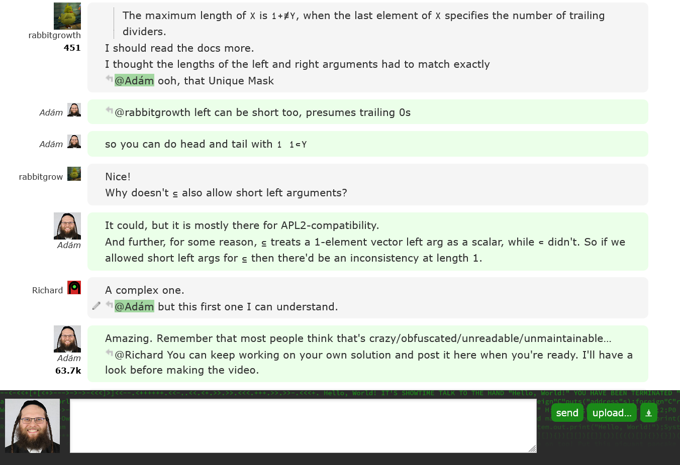
“Hacking” RIDE v4.5
This time, I didn’t need to modify source files, but rather found that RIDE was “vulnerable” (though not in a dangerous way) to CSS injection through its font input field. Making the font bold didn’t look right, as that would only smear the letters horizontally, but adding a “text stroke” had the desired effect. If you want your RIDE to resemble what you can see in the videos, set the APL font to SAX2')}.monaco-editor *{-webkit-text-stroke:.67px currentcolor}. With the visuals set, I recorded using OBS Studio and, on the rare occasion that I needed to edit something, I used DaVinci Resolve.
Concluding the Series
When we finished that last session, it felt rather anti-climactic, but I can look back on a very enjoyable time. And of course, the efforts that all participants put into this are not forgotten; we’ve got an amazing chat and video series that future APLers can enjoy. Thank you to everyone who contributed; chat participants, video commenters, colleagues (especially Brian Becker who authored all the problems), and most of all my wife, who often had to encourage me to record the next video(s) and also gave me the time and space to do so, even if it meant single-handedly keeping our children quiet. If you’re up for a marathon, you can watch the entire 22-hour series on YouTube, and APL Quest on the APL Wiki includes links to all the problems, chat sessions, code, and videos.
The section that is dedicated to the annual APL Problem Solving Competition is always one of my own favourite parts of a Dyalog user meeting, and the talks by the two winners this year were no exception. It is always a treat to hear about how the student winners are able to go from zero knowledge about APL to delivering very well designed, array-oriented, solutions in a few weeks, sometimes days!
This year, we were very pleased to have both the student grand prize winner Andrea Piseri and the professional winner Alexander Block present. Andrea is studying mathematics at Università degli Studi di Milano (University of Milan) and Alexander is an actuary at the Viridium Insurance Group in Germany.
Before Gitte Christensen presented the prizes to the winners and they gave their talks, our “Chief Problem Maker” Brian Becker gave us a brief history of the competition and overview of the contest website (which uses Dyalog-grown tools). He also mentioned that we are revising the format of the competition, most likely by running simpler/smaller problem sets at a higher frequency. We’ll be making official announcements about that early in 2024.
We started Wednesday with an update to the co-dfns project by Aaron Hsu. Aaron is trying to make APL more accessible to more people for tackling more problems. He explained how version 4 focusses on good performance on GPUs and detailed error reporting – including a parser that can be used for static analysis of APL code outside of Co-dfns – and how version 5 intends to target more platforms, improving integration of APL in other systems. There are even rumours of a JavaScript backend on the horizon! Dyalog available in the browser, wherever you go.
Brandon Wilson presents the challenges of parsing YAML
Brandon Wilson is a relative newcomer to APL. Although his main interest is in AI safety, he has significant experience in mainstream computer systems. This is part of what made him decide to write a YAML (YAML Ain’t Markup Language) parser in APL. Interestingly, most of the existing YAML parsers in use today fail some part of the test suite. This speaks to the complexity of the task and how there are many interactions between different parts of YAML that are not obvious. Brandon is hoping that writing a complete parser the APL way will lead to insights into the YAML specification that he can give back to the YAML community to help the specification developers better communicate what is needed to other parser maintainers.
Next, Josh David highlighted the huge demand for statistics in data science, machine learning, and the increase of data-driven decision-making in business. Although data preparation is easy in APL, he noted the lack of ready-made code for doing statistics. Simple summaries and linear regression take just a few primitives, but Josh showed us a couple of libraries for doing more complex statistical analysis. He demonstrated rapid iteration on multiple linear regression using KokoStats by Dr. Bill Koko, performing multiple tests and seeing the impact of the selected data on the predictive power of the regression model. In Professor Stephen Mansour’s TamStat package, the use of operators reduces the overall number of functions that users need to memorise, and a cross-platform graphical interface makes a great environment for exploring and learning statistics.
Jesús Galan Lopez returned to expand on something that he mentioned in his previous presentation – the modelling of grain growth in solid materials. Students at his university were tasked with reproducing models from published research. They wrote their solutions in Python because it was familiar to them, but Jesús wanted to see how array programming would compare. He found that his APL solution was generally shorter, cleaner, and faster. Of course, he had to compare more like-for-like programs by trying his solution in NumPy as well, and he found Dyalog had comparable performance.
Grand Prize winner Andrea Piseri
Then it was time for the presentation of prizes to winners of this year’s APL Problem Solving Competition. Brian Becker gave a brief history of the competition and overview of the contest website (which uses Dyalog-grown tools). He also announced future changes to the competition, such as quarterly sets of Phase-1-style one-liner problems. Gitte then presented certificates to the student grand prize winner, Andrea Piseri, and professional winner, Alexander Block.
Alexander was first to introduce himself – he is an actuary using APL to solve problems, working in insurance companies in Germany – and talk us through a couple of his solutions. Having used Haskell, he is a big fan of point-free (tacit) programming, and liked his use of the over operator (⍥) in his solution to the Risk attack problem from phase 1 (problem 5).
Professional winner Alexander Block
Andrea Piseri is a mathematics student with a particular interest in abstract algebra and mathematical logic, as well as a programming language enthusiast. Coming from the functional programming world, Andrea first solved the DNA reading frames problem (phase 2, problem 1, task 5) using the “flatmap” pattern, but then came up with another solution leveraging comparison and interval-index to process the whole input at once. When tackling the “make change” problem (phase 2, problem 2, task 3) he was surprised to find APL was not so opinionated and that he could quite easily map iterative and recursive patterns from Haskell onto dfns.
This afternoon was the annual Viking Challenge, and this year the team from Midgaard Event set up a thrilling mystery in which we were split into teams to solve a variety of puzzles. The individual puzzles offered a range of challenges to suit all participants, with the ultimate challenge being to piece clues together in a process of elimination. There was temptation to write an APL program to solve the problem, but it was resisted as nine of the twelve teams managed to work out the solution with pen and paper. Eyes rolled with chagrin all around the auditorium when it was announced that the winning team was the team that included both Gitte and Stine!
By: Stefan Kruger Stefan works for IBM making databases. He tries to learn at least one new programming language a year, and a few years ago he got hooked on APL and participated in the competition. This is his perspective on some solutions that the judges picked out – call it the “Judges’ Pick”, if you like; smart, novel, or otherwise noteworthy solutions that can serve as an inspiration.
Congratulations to all the winners of the 2021 APL Problem Solving Competition (you can learn more about the phase 2 winners in this article) and well done to Dzintars Klušs who won the Grand Prize. At the recent Dyalog ’21 user meeting, we got to enjoy the runner-up, Victor Ogunlokun, walking us through his solutions live.
In this post I’ll go through some great solutions that were submitted (and some that weren’t submitted) to the Phase I problems so that we can all marvel in the ingenuity and perhaps learn a thing or two. If you’re feeling inspired by the end, go ahead and participate in this year’s round which just launched.
If you’re new to the APL Problem Solving Competition, Phase I problems tend to be short and the expectation is that solutions will be “one-liners” (dfns). However, although it might seem like it from some of the solutions here, this isn’t a code golf competition! Solutions are judged holistically: do they solve the problem, are they efficient, and are they clear? Even though a few test cases are given, there is no guarantee that your solution is correct just because it works for the example data. The judging process involves running the code on many hidden test cases too. Crucially, just because your code is accepted, it doesn’t necessarily mean that you’ll get full marks.
Something from the excellent Project Rosalind problem collection, the task is to compute the combined percentage of guanine (G) and cytosine (C) in a given DNA-string.
Efficiency can vary a lot, depending on whether summation or multiplication (or even division!) is performed first. Some solutions were also leading-axis oriented.
Here’s my solution:
      {100×(+⌿⍵∊'CG')÷≢⍵} 'ACGTACGTACGTACGT'
50
which several competitors made more tacit with:
      {100×(+⌿÷≢)⍵∊'GC'} 'ACGTACGTACGTACGT'
50
or even went further:
      (100×≢÷⍨1⊥∊∘'GC') 'ACGTACGTACGTACGT'
50
If you’re unfamiliar with the 1⊥ trick, it’s a way of summing a vector:
      1⊥6 3 9 8 12 62
100
It’s perhaps not immediately obvious why this should work. Here’s one explanation. Assume we want to sum the vector 1 0 2 0 0. We can do this in a very convoluted way by using a sum inner product with a vector of exponentials: [14, 13, 12, 11, 10]:
      (1*4 3 2 1 0)+.×1 0 2 0 0
3
If we expand the exponentials to the left we get a vector of 1s. We can then break apart the inner product by turning +. to a +⌿ to the left:
      +⌿1 1 1 1 1×1 0 2 0 0
3
This is the textbook definition of 1⊥! Look:
      1⊥1 0 2 0 0
3
which, to be clear, is just the sum-reduce-first:
      +⌿1 0 2 0 0
3
Using 1⊥ to sum has two advantages over the more obvious formulation +⌿. Firstly, it’s easier to use in tacit formulations as it doesn’t require an operator, and secondly, it’s usually faster. The reasons for it being quicker is somewhat beyond the scope of this post, but it’s to do with 1⊥ making no guarantees about the ordering of operations, meaning that the interpreter is free to vectorise more efficiently.
Problem 2: Index-Of Modified
This problem wanted us to write a function that behaves like the APL Index Of function R←X⍳Y except that it should return 0 for elements of Y not found in X.
I wrote:
      p2 ← {0@((≢⍺)∘<)⊢⍺⍳⍵}
      2 3 p2 ⍳5
0 1 2 0 0
which is basically saying “change all instances of numbers greater than the length of the argument to zero”, which is how X⍳Y presents values that are not found.
Some very different solutions were submitted, for example:
      p2 ← ⍳|⍨1+≢⍤⊣
      2 3 p2 ⍳5
0 1 2 0 0
which is simply:
      p2 ← {(1+≢⍺)|⍺⍳⍵} ⍝ dfn of the above
      2 3 p2 ⍳5
0 1 2 0 0
Another option would have been to multiply ⍺⍳⍵ with ≢⍺, although no-one submitted exactly this:
      p2 ← ≢⍤⊣(≥×⊢)⍳
      2 3 p2 ⍳5
0 1 2 0 0
which could have been written explicitly as:
      p2 ← {m×(≢⍺)≥m←⍺⍳⍵} ⍝ dfn of the above
      2 3 p2 ⍳5
0 1 2 0 0
Problem 3: Multiplicity
Write a function that:
has a right argument Y which is an integer vector or scalar
has a left argument X which is also an integer vector or scalar
finds which elements of Y are multiples of each element of X and returns them as a vector (in the order of X) of vectors (in the order of Y).
although no-one actually submitted that, to everyone’s credit.
Problem 4: Square Peg, Round Hole
Write a function that:
takes a right argument which is an array of positive numbers representing circle diameters
returns a numeric array of the same shape as the right argument representing the difference between the areas of the circles and the areas of the largest squares that can be inscribed within each circle.
I had to read that many times before it sank in. The key to achieve something snappy is to really work through the maths until it is as compact as possible, which, if you’re anything like me, you didn’t bother to do.
My attempt was:
p4 ← {(○2*⍨⍵÷2)-2÷⍨⍵*2}
but there are much neater solutions if you did your homework. Here’s one that no-one found:
p4 ← (○-+⍨)4÷⍨×⍨
and a nice explicit version:
p4 ← {⍵×⍵×0.5-⍨○÷4}
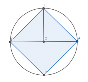
which can be derived from this simplified mathematical expression, suggested by Rodrigo:
Explanation: The area of the circle is ○r*2, which is ○(⍵÷2)*2, in turn equivalent to ⍵×⍵×○÷4. The area of the square [ABCD] is twice the area of the triangle [ABC]. Given that the area of the triangle is 0.5×⍵×⍵÷2, the area of the square becomes 0.5×⍵×⍵. Putting both together, we get (⍵×⍵×○÷4)-⍵×⍵×0.5, the same as ⍵×⍵×(○÷4)-0.5, which is ⍵×⍵×0.5-⍨○÷4.
Problem 5: Rect-ify
For this problem, we were asked to plant a number of trees in a rectangular pattern with complete rows and columns, meaning all rows have the same number of trees. That rectangular pattern also needed to be as “square as possible”, meaning there is a minimal difference between the number of rows and columns in the pattern.
Here’s a smart solution, based on the observation that the “most square” choice must have one factor being the largest factor less than or equal to the square root:
p5 ← {N,⍵÷1⌈N←⌈/0,⍵∨⍳⌊⍵*÷2}
This solution works well on large numbers of trees, too:
So is one solution better than the other? Well, they both work correctly, but one is a lot faster than the other. Do you want to guess which was faster before we test it?
Surprised? I was! So, what is going on here? The non-recursive solution relies on a rather crude way to find the factors, which is a fairly large number to factorise even if it only needs to go up to the square root. The recursive version just tries each number in turn, up to the square root.
Can we be even smarter? This version was offered up by APL Orchard regular @rak1507:
Basically, (⊢∨⍳) is neat as a code-golf trick, but not great in terms of efficiency.
Problem 6: Fischer Random Chess
According to Wikipedia, Fischer random chess is a variation of the game of chess invented by former world chess champion Bobby Fischer. Fischer random chess employs the same board and pieces as standard chess, but the starting position of the non-pawn pieces on the players’ home ranks is randomised, following certain rules.
White’s non-pawn pieces are placed on the first rank according to the following rules:
the Bishops must be placed on opposite-colour squares
the King must be placed on a square between the rooks.
The task was to write a function that verifies that a given board placement is valid according to these rules.
This was my solution for this:
q6 ← {(1=+/(⍵⍳'K')>⍸'R'=⍵)∧1=+/2|⍸'B'=⍵}
but there was a lot of variety in the solutions submitted to this problem. For example:
q6i ← {≠/2|⍸'B'=⍵}∧'RKR'≡∩∘'RK' ⍝ Intersection
q6ii ← {(≠/2|⍸'B'=⍵)∧1=(⍸'R'=⍵)⍸⍵⍳'K'} ⍝ Interval index
q6w ← {(≠/2|⍸'B'=⍵)∧≠/(⍸'K'=⍵)<⍸'R'=⍵} ⍝ Where (similar to mine above)
The fork ⍉,[0.5]⌽ takes the argument matrix – a square array of rank-2, shape A A – and returns an array of rank-3, shape 2 A A, where the first cell is the transposed original array and the second is the original array with its rows reversed:
We only need to know about the main diagonal of each cell; as you can see, the main diagonal in the second cell is the reverse diagonal of the first cell. We can extract both diagonals with a single dyadic transpose:
      1 2 2⍉(⍉,[0.5]⌽) magic
4 5 6
2 5 8
The same result can be achieved using slightly less showy ⍤ instead, which has the same byte count but is a little easier to understand when first seen:
      1 1⍉⍤2(⍉,[0.5]⌽) magic ⍝ Diagonals of each major cell love ⍤
4 5 6
2 5 8
The remaining part of the tacit formulation untangles easily. Impressive and creative.
      {1=≢∪+⌿⍵,⍥{(1 1⍉⍵),⍵}⌽⍵} magic ⍝ Length of vector of unique values = 1?
1
In summary, there are two things to note here: using ⍥ to get both diagonals and the use of 1=≢∘∪ to check that all items are equal. If you attended the APL Seeds ’21 conference last March, you’ll recognise this as one of the many ways of solving this problem that Conor Hoekstra presented – see https://dyalog.tv/APLSeeds21/?v=GZuZgCDql6g to watch his presentation.
Any solution that makes use of both of my favourite glyphs (⍤ and ⍥) is a winner in my book.
Problem 8: Time to Make a Difference
Write a function that:
has a right argument that is a numeric scalar or vector of length up to 3, representing a number of [[[days] hours] minutes] – a single number represents minutes, a 2-element vector represents hours and minutes, and a 3-element vector represents days, hours, and minutes
has a similar left argument, although not necessarily the same length as the right argument
returns a single number representing the magnitude of the difference between the arguments in minutes.
Here’s a cool version (several submissions were similar):
p8 ← |-⍥(1 24 60⊥¯3∘↑)
Nothing too mysterious here. A slight complication is the need to handle a right argument that can be a scalar or a vector of length 2 or 3. The decode function ⊥ expects the argument vector to always be length 3, so we use the take function, dyadic ↑, with ¯3 as the left argument to ensure that the argument is always a vector of the correct length, padding from the left with zeros as required. The mixed radix vector 1 24 60 as the left argument to decode converts to minutes.
Problem 9: In the Long Run
Write a function that:
has a right argument that is a numeric vector of 2 or more elements representing daily prices of a stock
returns an integer singleton that represents the highest number of consecutive days where the price increased, decreased, or remained the same, relative to the previous day.
I’d like to compare and contrast two solutions, neither of which are tacit for a change:
Starting with the first of the two (p9a), from the right, we use a windowed difference reduction to calculate pairwise differences:
      2-/1 3 5 6 6 6 6 6 3 2 1
¯2 ¯2 ¯1 0 0 0 0 3 1 1
and then apply the direction function, monadic ×, to turn this into a vector of ¯1, 0 and 1 if the corresponding item is negative, zero or positive respectively:
      ×2-/1 3 5 6 6 6 6 6 3 2 1
¯1 ¯1 ¯1 0 0 0 0 1 1 1
Another pairwise windowed reduction, this time with ≠, gives us the points of change:
      2≠/×2-/1 3 5 6 6 6 6 6 3 2 1
0 0 1 0 0 0 1 0 0
Prepending a 1, this Boolean vector can be used as the left argument to partitioned enclose, ⊂; a common pattern. But what of the right argument? We can use the same vector as the right argument by using a clever commute, ⍨:
      ⊢m←⊂⍨1,2≠/×2-/1 3 5 6 6 6 6 6 3 2 1 ⍝ Commute to use the same argument left and right
┌─────┬───────┬─────┐
│1 0 0│1 0 0 0│1 0 0│
└─────┴───────┴─────┘
What remains is to find the longest cell in this vector. We could do ⌈/≢¨, but instead this submission found the length of the transpose-mix:
      ≢⍉↑ m
4
A code-golfer’s trick shot, perhaps, and somewhat dubious in terms of efficiency, but certainly cute. If you don’t see why it works, work it through right to left!
The second solution (p9b) uses a lot of the same ideas, but this time we add a 1 to the end of the points-of-change vector:
and use where, monadic ⍸, to get the indices, prepending a 0 so that we can calculate the length of each segment:
      {0,⍸1,⍨2≠/×2-/⍵}1 3 5 6 6 6 6 6 3 2 1
0 3 7 10
The pairwise difference now represents the length of each segment, and by using a negative window we can commute each pair to get a positive number out for each pair:
      {¯2-/0,⍸1,⍨2≠/×2-/⍵}1 3 5 6 6 6 6 6 3 2 1
3 4 3
and so, for the maximum:
      {⌈/¯2-/0,⍸1,⍨2≠/×2-/⍵}1 3 5 6 6 6 6 6 3 2 1
4
Shall we race them? Of course!
      data ← 10000?10000
      cmpx 'p9a data'
  p9a data → 2.7E¯4 |   0% ⎕⎕⎕⎕⎕⎕⎕⎕⎕⎕⎕⎕⎕⎕⎕⎕⎕⎕⎕⎕⎕⎕⎕⎕⎕⎕⎕⎕⎕⎕⎕⎕⎕⎕⎕⎕⎕⎕⎕⎕
  p9b data → 2.1E¯5 | -92% ⎕⎕⎕
The second version is faster for several reasons. We suspected already that the ‘cute’ way to find the longest vector in a nested vector was likely to be slow, as it has to create a huge matrix first, chasing pointers. The second version uses flat numeric vectors throughout, and cuts the work considerably by using where initially to do length calculations on the shorter vector of indices. Flat is fast.
Problem 10: On the Right Side
Write a function that:
has a right argument T that is a character scalar, vector or vector of character vectors/scalars
has a left argument W that is a positive integer specifying the width of the result
returns a right-aligned character array R of shape ((2=|≡T)/≢T),W meaning that R is one of the following:
a W-wide vector if T is a simple vector or scalar
a W-wide matrix with the same number rows as elements of T if T is a vector of vectors/scalars
if an element of T has length greater than W, truncate it after W characters.
The last point is perhaps a bit misleading, but the intention is clear from one of the examples given:
In this case, “truncate after W characters” means “remove from the left”.
Conceptually, we need to (over)take W characters from the right of each element and mix that into a rank-2 array. To make it work for the edge cases, we should ensure that we can always treat the right argument as a vector of character vectors, using nest, monadic ⊆. This works because if we take more characters than the vector contains, it gets padded using a character-vector’s prototype element, a space.
            8 {↑(-⍺)↑¨⊆⍵} 'Longer Phrase' 'APL' 'Parade'
r Phrase
     APL
  Parade
An equivalent tacit formulation would be:
            8 (↑-⍤⊣↑¨⊆⍤⊢) 'Longer Phrase' 'APL' 'Parade'
r Phrase
     APL
  Parade
Here’s a slight variation:
            8 {⌽⍉⍺↑⍉↑⌽¨⊆⍵}'Longer Phrase' 'APL' 'Parade'
r Phrase
     APL
  Parade
This starts by reversing each cell, then applies a mix and transpose. We then take items from the left before backing out of the transpose and reverse by applying them again.
It can be done in a flatter manner, too:
            8{⍉(-⍺)↑⍉(⊆⍵)⌽∘↑⍨(⊢-⌈/)≢¨⊆⍵} 'Longer Phrase' 'APL' 'Parade'
r Phrase
     APL
  Parade
If we flip the selfie and add a few spaces it gets a bit easier to see what’s going on:
From the right, we turn our input into a character array and then Rotate each row by its length minus the length of the longest row, which implements the right alignment:
The complex, flat version wins, but not by a significant amount.
With that we’ve reached the end. A nice set of problems, with a lot of creative solutions submitted. Watch this space for a review of the Phase II problems…
With Dyalog’s APL Problem Solving Competition 2021 in full swing, it’s time to highlight some of the excellent solutions that were submitted to last year’s edition.
Stefan Kruger works for IBM making databases. While he tries to learn at least one new programming language a year, he got hooked on APL and participated in the competition. This is his perspective on some solutions that the judges picked out – call it the “Judges’ Pick”, if you like; smart, novel, or otherwise noteworthy solutions that can serve as an inspiration.
I’ll show a cool solution or two to each Phase II problem and dive into the details of a couple. If you need to refresh your memory with what the problems looked like, there’s a PDF of the Phase II problems.
Oh, and note that at the time of writing there is still plenty time to take part in the current edition of the competition (and really, who knew bowling was so complicated?) – there are some juicy cash prices to be won.
Problem 1: Take a Dive (1 task)
Level of Difficulty: Low
So let’s kick off with problem 1. The task was to calculate the score of an Olympic dive, consisting of a technical difficulty rating and a vector containing either 3, 5 or 7 judges’ scores. Only the central three ordered judges’ scores should be considered, which should be summed and multiplied by the technical difficulty rating.
Here is a cunning trick that wasn’t at all obvious:
∇ score←dd DiveScore scores;sorted;cenzored;rotator
  ⍝ 2020 APL Problem Solving Competition Phase II
  ⍝ Problem 1, Task 1 - DiveScore

  sorted←{⍵[⍋⍵]}scores

  ⍝  0 1 2 rotates score indexes to 123, 23451 or 3456712
  ⍝  So three center values always goes first
  ⍝  51 = (0 1 2∧.= 3 5 7 ∘.|⍳100) ⍳ 1
  rotator←51

  cenzored←3↑rotator⌽sorted
  score←⍎2⍕dd+.×cenzored
∇
This contestant figured out that if a vector of length 3, 5 or 7 is rotated 51 steps, then the original central three items will always end up at the beginning. No, really. It turns out that 51 is the first number X such that 0 1 2≡3 5 7|X. They tabulated the options and picked the first solution, guessing that it’d be less than 100:
      ⍸0 1 2∧.=3 5 7∘.|⍳100
51
But there is another way – this is one of those situations where the Chinese Remainder Theorem comes in handy, especially since it’s available on APLcart:
If you figured that out, award yourself a well-deserved pat on the back. For us mortals, we probably all did something rather more pedestrian:
DiveScore ← {
    d ← 2-2÷⍨7-≢⍵       ⍝ How many items should we drop each side?
    ⍺+.×(-d)↓d↓⍵[⍋⍵]
}
Problem 2 – Another Step in the Proper Direction (1 task)
Level of Difficulty: Medium
Problem 2 builds upon Problem 5 from Phase I. In short, we are asked to write a function Steps that takes a two-element vector to the right, defining a start and end value, and an optional left integer argument that tweaks how we generate values from start to end. The complexity here comes from the many combinations of behaviours from what exactly is given as the left argument: integer or float? positive or negative? Also, the range must be inclusive, even if a floating-point step size means that the end point is overshot. I took this on thinking it would be trivial – it wasn’t.
Here’s a great solution that manages to combine this functionality with a call to a single dfn:
∇ steps←{p}Steps fromTo;segments;width
  width ← |-/fromTo
  :If 0=⎕NC'p' ⍝ No left argument: same as Problem 5 of Phase I
      segments ← 0,⍳width
  :ElseIf p0 ⍝ p is the step size
      segments ← p {⍵⌊⍺×0,⍳⌈⍵÷⍺} width
  :ElseIf p=0 ⍝ As if we took zero step
      segments ← 0
  :EndIf
  ⍝ Take into account the start point and the direction.
  steps ← fromTo {(⊃⍺)+(-×-/⍺)×⍵} segments
∇
I ended up with something more convoluted, with a few ugly special cases, and shamelessly borrowing from dfns.iotag:
Steps ← {
    range ← {
        r ← ⍺-s×⎕IO-⍳⌊1-(⍺-⊃⍵)÷s←×/1↓⍵,(⍺>⊃⍵)/¯1 ⍝ "inspired" by dfns.iotag
        (⊃⍵)≠⊃⊖r: r,⊃⍵ ⋄ r   ⍝ Ensure endpoint is included – yeuch :(
    }
    ⍺ ← ⍬
    (b e) ← ⍵
    ⍺≡⍬: b range e        ⍝ No ⍺
    ⍺=0: b                ⍝ Zero step; return start point
    ⍺>0: b range e ⍺      ⍝ Positive ⍺
    len ← (e-b)÷count←⌊-⍺ ⍝ Negative ⍺
    len=0: b/⍨1+count
    b range e len
}
Problem 3 – Past Tasks Blast (1 task)
Level of Difficulty: Medium
The task here was to scrape the Dyalog APL Problem Solving Competition webpage to extract all links to PDF files. We get the suggestion to use either Dyalog’s HttpCommand or shell out to a system mechanism for fetching a web page.
To use HttpCommand, we first need to load it:
      ]load HttpCommand
#.HttpCommand
Here’s a slightly tweaked competition submission, showing great flair in how to process XML:
PastTasks ← {
    url ← ⍵
    r ← (HttpCommand.Get url).Data  ⍝ get page contents
    (d n c a t) ← ↓⍉⎕XML r          ⍝ depth; name; content; attributes; type
    (k v) ← ↓⍉ ⊃⍪/ ((,'a')∘≡¨n)/a   ⍝ extract key-value pairs of <a> elements
    urls ← ('href'∘≡¨k)/v           ⍝ get URLs
    pdfs ← ('.pdf'∘≡¨¯4↑¨urls)/urls ⍝ filter .pdfs
    base ← ⊃⌽⊃('base'∘≡¨n)/a        ⍝ base URL
    base∘,¨pdfs
}
The problem statement suggests that a regex-based solution might be tolerable. Here’s a stab at that approach:
PastTasks ← {
    body ← (HttpCommand.Get ⍵).Data
    pdfs ← '<a href="(.+?\.pdf)"'⎕S'\1'⊢body
    base ← '<base href="(.+?)"'⎕S'\1'⊢body
    base,¨pdfs
}
So which is the “better” solution? Well, the first approach has a number of advantages: firstly, is much more robust (provided that the web page is valid XHTML, which we are told is a given), meaning that we can abdicate responsibility for dealing with markup quirks (single vs double quotes, whitespace etc) to the built-in ⎕XML system function, and secondly, there is that (in)famous quote from Jamie Zawinski:
Some people, when confronted with a problem, think “I know, I’ll use regular expressions.” Now they have two problems. – jwz
Mixing in a liberal helping of regular expressions in with APL is perhaps not helping APL’s unfair reputation for being write-only.
However, when dealing with patterns in textual data, as we unquestionably are here, regular expressions – even in a powerful language like APL – are sharp tools that are hard to beat, and any programmer worth their salt owes it to themselves to master them. In the case above, had the data not neatly been parseable as XML, it would have been more awkward to solve a problem like this relying only on APL primitives.
Problem 4 – Bioinformatics (2 tasks)
Level of Difficulty: Medium
The two tasks making up Problem 4 are borrowed from Project Rosalind, which is a Bioinformatics problem collection that often has great APL affinity:
and a hint that one benefits from understanding modular multiplication, as this isn’t built into Dyalog APL.
Here is a great example:
revp ← {                    ⍝ r ← revp dna
   dnaNum ← 'ACGT'⍳⍵        ⍝ Convert to 1..4 so that A+T = C+G = 5
   FindRevp ← {             ⍝ Given chunk size, extract positions and build the output format
       chunks ← ⍵,/dnaNum
       isRevp ← (⊢≡5-⌽)¨chunks
       ⍵,⍨⍪⍸isRevp
   }
   ⊃⍪/FindRevp¨4 6 8 10 12  ⍝ Test against all chunk sizes and collect results
}
sset ← {          ⍝ r←sset n
   bin ← 2⊥⍣¯1⊢⍵  ⍝ Binary digits
   arr ← ⌽2*bin   ⍝ Repeated squaring: Starting from MSB and 1, square ⍵, multiply ⍺, modulo m
   mod ← 1000000
   {mod|⍺×⍵*2}/arr,1
}
This contestant also saw fit to include their test suite; a nice touch! Roger Hui’s version of assert has become the de facto standard, and the contestant puts it to good use:
Problem 5 is some hedge fund maths, or something where my eyes glazed over before I fully understood the ask. What is this, K‽
This solution is impressively compact – I removed the comments to highlight the APL artistry on display: no less than three scans, count ’em!
rr ← {AR×+\⍺÷AR←×\1+⍵}
pv ← {+/⍺÷×\1+⍵}
Here’s how the competitor outlined how their solution works:
This can be calculated elegantly with the following operations:
Find the accumulated interest rate (AR) for each term (AR←×\1+⍵).
Deprecate the cashflow amounts by dividing them by AR. This finds the present value of all the amounts.
Accumulate all the present values of the amounts to find the total present value at each term.
Multiply by AR to find future values at each term.
This way the money that was invested or withdrawn in a term is not changed for that term, but the money that came from the previous terms is multiplied by the current interest rate for each term arriving to the correct recurrent relation:
Mail merge – gotta love it. Your spam folder is full of bad examples of this: “Dear $FIRSTNAME, do you want to purchase a bridge?” We’re given a template file with patterns such as @firstname@ which are to be replaced with values stored in a JSON file. Here’s a smart approach from a competitor who knows their way around the @ operator:
The key insight here is that since each template starts and ends with the same marker, we can partition the data on sections beginning with @ and then we’ll have a vector where every other element is a template to be substituted. Here’s an example of this:
      ↑('@'(1↓¨=⊂⊢) '@title@ @firstname@ @lastname@, would you be interested in the Brooklyn Bridge?') (1 0 1 0 1 0)
┌─────┬─┬─────────┬─┬────────┬─────────────────────────────────────────────────┐
│title│ │firstname│ │lastname│, would you be interested in the Brooklyn Bridge?│
├─────┼─┼─────────┼─┼────────┼─────────────────────────────────────────────────┤
│1    │0│1        │0│1       │0                                                │
└─────┴─┴─────────┴─┴────────┴─────────────────────────────────────────────────┘
I added the second row for clarity to show the alternating templates. Cool, huh? However, this only works correctly if the data leads with a template. Consider:
      '@'(1↓¨=⊂⊢) 'Dear @firstname@ @lastname@, or maybe the Golden Gate?'
┌─────────┬─┬────────┬───────────────────────────┐
│firstname│ │lastname│, or maybe the Golden Gate?│
└─────────┴─┴────────┴───────────────────────────┘
We still have the alternating templates, but the prefix (Dear ) is lost. We can tweak the Merge function a bit to cater for this if we need to:
Merge ← {
    templateFile ← ⍺
    jsonFile ← ⍵
    template ← ⊃⎕NGET templateFile
    ns ← ⎕JSON⊃⎕NGET jsonFile
    first ← templ⍳'@'
    first>≢templ: templ    ⍝ No templates at all
    prefix ← first↑templ   ⍝ Anything preceding the first '@'?

    getValue ← {
        0=⍴⍵:,'@'   ⍝ '@@'         → ,'@'
        6::'???'    ⍝ ~⍵∊ns.⎕NL ¯2 → '???'
        ⍕ns⍎⍵       ⍝  ⍵∊ns.⎕NL ¯2 → ⍕ns.⍵
    }
    ∊prefix,getValue¨@(⍴⍴1 0⍨)'@'(1↓¨=⊂⊢)template
}
Now, the competition is pitched such that “proper array solutions” are preferred – and for good reasons, most of the time. However, it’s hard to overlook some industrial regex action in this case. Strictly for Perl-fans:
Problem 7 had us learning more about bar codes than we ever thought necessary. Read them, write them, verify them, scan them – forwards and backwards no less. Good scope for stretching your array muscles on this one. The eagle-eyed amongst you may have spotted that the verification aspect is a simplified version of Luhn’s algorithm, which a certain Morten Kromberg used to illustrate APL’s array capabilities at JIO a while back.
Here’s a good solution:
CheckDigit ← (10|∘-+.×∘(11⍴3 1))          ⍝ Computes the check digit for a UPC-A barcode.

UPCRD ← 114 102 108 66 92 78 80 68 72 116 ⍝ Right digits of a UPC-A barcode, base 10.
bUPCRD ← ⍉2∘⊥⍣¯1⊢UPCRD                    ⍝ Bit matrix with one right digit per row.
WriteUPC ← {
   ⍝ Writes the bits of a UPC-A barcode.
   ~((11∘=≢)∧(∧/0∘≤∧≤∘9))⍵: ¯1            ⍝ Check for simple errors
   b ← bUPCRD[⍵,CheckDigit ⍵;]
   1 0 1, (,~6↑b), 0 1 0 1 0, (,6↓b), 1 0 1
}
ReadUPC ← {
   ⍝ Reads a UPC-A barcode into its digits.
   ~(∧/0∘≤∧≤∘1)⍵: ¯1                 ⍝ Input isn't a bit vector
   95≠≢⍵: ¯1                         ⍝ Number of bits must be 95
   (b l m r e) ← ⍵ ⊂⍨ (∊¯1∘↓,⌽) (3↑1)(42↑1)(5↑1)

   b ∨⍥(≢∘1 0 1) e: ¯1               ⍝ Wrong patterns for the guards
   m≢0 1 0 1 0: ¯1
   bits ← ↓12 7⍴ l,r
   C ← (↓bUPCRD)∘⍳ ~@(⍳6)            ⍝ Convert bits to digits
   tf ← ~∧/10 > nums ← C bits        ⍝ Should we try flipping the bits?
   nums ← (nums×1-tf) + tf×C⌽↓⌽↑bits
   ∨/10=nums: ¯1                     ⍝ Bits simply aren't right
   (¯1↑nums)≠CheckDigit 11↑nums: ¯1  ⍝ Bad check digit
   nums
}
Problem 8 – Balancing the Scales (1 task)
Level of Difficulty: Hard
Our task is to partition a set of numbers into two groups of equal sum if this is possible, or return ⍬ if not. This is a well-known NP-complete problem called The Partition Problem and, as such, has no polynomial time exact solutions. The problem statement indicates that we only need to consider a set of 20 numbers or fewer, which is a bit of a hint on what kind of solution is expected.
This problem, in common with many other NP problems, also has a plethora of interesting heuristic solutions: polynomial algorithms that whilst not guaranteed to always find the optimal solution will either get close, or be correct for a significant subset of the problem domain in a fraction of the time the exact algorithms would take.
However, it’s clear that Dyalog expects us to give an exact solution, and has given us an upper bound on the input data length. Finally, we’re offered the cryptic advice that
Understanding the nuances of the problem is the key to developing a good algorithm.
Yes, thank you, master Yoda.
Here’s a great, efficient solution:
Balance←{
   sum←1⊥⍵
   2|sum: ⍬   ⍝ Lists with an odd sum cannot be split into equal parts.
   halfsum←sum÷2

   ⍝ A partitioning method based on the algorithm by Horowitz and Sahni.
   ⍝ The basic idea of the algorithm is to split the input into two parts,
   ⍝ and then generate all subset sums for these parts. Then the problem
   ⍝ becomes finding a sum of two subset sums from different parts
   ⍝ equal to the desired value. Instead of sorting the sums and comparing
   ⍝ them like in the original algorithm, standard APL searching primitives
   ⍝ ∊ and ⍳ are used. Another key idea is to generate the subset sums
   ⍝ in a specific order, so that the nth subset sum in the vectors a and b
   ⍝ is the sum of the elements chosen by the binary representation of n.
   ⍝ This means that we can get the elements of the solution sum
   ⍝ without having to generate anything but the sums.
   horowitzsahni←{
       s←⍵(↑{⍺⍵}↓)⍨⌊2÷⍨≢⍵                          ⍝ Split the input.
       a b←⊃¨(⊢,+)/¨s,¨0                           ⍝ Generate the subset sums.
       indexes←a {(⊢,⍵⍳⍺⌷⍨(≢⍺)⌊⊢)1⍳⍨⍺∊⍵} halfsum-b ⍝ Search for solution indexes.
       indexes[2]>≢b: ⍬
       ⍵ {(⍺/⍨~⍵)(⍵/⍺)} ∊(2⍴¨⍨≢¨s)⊤¨indexes-1      ⍝ Get the solution from the indexes.
   }

   ⍝ A simple exhaustive search. It uses the same binary representation
   ⍝ idea as the horowitzsahni function.
   exhaustive←{
       i←halfsum⍳⍨⊃(⊢,+)/⍵,0
       i>2*≢⍵: ⍬
       ⍵ {(⍺/⍨~⍵)(⍵/⍺)} (2⍴⍨≢⍵)⊤i-1
   }

   ⍝ The exhaustive method performs better than the Horowitz-Sahni method
   ⍝ for small input sizes. 14 seems to be a reasonable cutoff point.
   14>≢⍵: exhaustive ⍵
   horowitzsahni ⍵
}
There are a number of clever touches here – there are actually two different solutions, an exhaustive search and an implementation of the algorithm due to Horowitz and Sahni, which, although still exponential, is known to be one of the fastest for certain subsets and input sizes. A switch based on input size checks for the crossover point and chooses the fastest option. And this is fast – five times faster than that of the Grand Prize winner, and four orders of magnitude faster than the slowest solution.
Such a performance spread is intriguing, so there are clearly lessons to be learned here. When I tried this problem, I ended up with a pretty straight-forward (a.k.a. naive) brute force search:
Balance ← {⎕IO←0
    total ← +/⍵
    2|total: ⍬             ⍝ Sum must be divisible by 2
    psum ← total÷2         ⍝ Our target partition sum
    bitp ← ⍉2∘⊥⍣¯1⍳2*≢⍵    ⍝ All possible bit patterns up to ≢⍵
    idx ← ⍸<\psum=bitp+.×⍵ ⍝ First index of partition sum = target
    ⍬≡idx: ⍬               ⍝ If we have no 1s, there is no solution
    part ← idx⌷bitp        ⍝ Partition corresponding to solution index
    (part/⍵)(⍵/⍨~part)     ⍝ Compress input by solution pattern and inverse
}
If you come to APL from a scalar language, that approach must seem incredibly wasteful: make all bit patterns. Try all sums. Search for the right one, if it exists. But as it turns out, this is APL home turf advantage. Let’s try to demonstrate this point. If you did this “loop and branch”, you’d iterate over the bit patterns and stop once you find the first solution – in fact, for the test data in the problem specification, the first solution appears at around the 1500th bit pattern if you generate them as I do above. The vector version would need to consider the whole space of around
      ¯1+2*20
1048575
a million or so, so quite a difference. Surely, in this case the scalar approach should be way faster? Only one way to find out. We can make a scalar version in several ways – here’s the “Scheme” version:
BalanceScalar ← {⎕IO←0     ⍝ Warning: this is not the APL Way, as we shall see.
    total ← +/⍵
    2|total: ⍬             ⍝ Sum must be divisible by 2
    psum ← total÷2         ⍝ Our target partition sum
    data ← ⍵
    bitp ← ↓⍉2∘⊥⍣¯1⍳2*≢⍵   ⍝ Pre-compute the bit patterns
    {                      ⍝ Try one sum after the other, halt on first solution
        0=⍵: ⍬
        patt ← ⍵⊃bitp
        psum=patt+.×data: (patt/data)(data/⍨~patt) ⍝ Exit on first solution found
        ∇¯1+⍵
    } ¯1+≢bitp
}
Dyalog’s got game when it comes to tail call optimisation, right? OK, let’s race:
      'cmpx'⎕CY'dfns'
      d ← 10 81 98 27 28 5 1 46 63 99 25 39 84 87 76 85 78 64 41 93
      cmpx 'Balance d' 'BalanceScalar d'
  Balance d       → 2.7E¯2 |   0% ⎕⎕⎕⎕⎕⎕⎕⎕⎕⎕⎕⎕⎕⎕⎕⎕⎕⎕⎕⎕⎕⎕⎕⎕⎕⎕⎕⎕
* BalanceScalar d → 3.9E¯2 | +43% ⎕⎕⎕⎕⎕⎕⎕⎕⎕⎕⎕⎕⎕⎕⎕⎕⎕⎕⎕⎕⎕⎕⎕⎕⎕⎕⎕⎕⎕⎕⎕⎕⎕⎕⎕⎕⎕⎕⎕⎕
Vectorisation, Boolean vectors and primitive functions wins the day. We didn’t go completely scalar, to be fair, as we still pre-computed all the binary patterns.
But back to the task at hand – let’s pit ourselves against the intellectual might of Horowitz and Sahni:
horowitzsahni←{
    sum←1⊥⍵
    2|sum: ⍬   ⍝ Lists with an odd sum cannot be split into equal parts.
    halfsum←sum÷2
    s←⍵(↑{⍺⍵}↓)⍨⌊2÷⍨≢⍵                          ⍝ Split the input.
    a b←⊃¨(⊢,+)/¨s,¨0                           ⍝ Generate the subset sums.
    indexes←a {(⊢,⍵⍳⍺⌷⍨(≢⍺)⌊⊢)1⍳⍨⍺∊⍵} halfsum-b ⍝ Search for solution indexes.
    indexes[2]>≢b: ⍬
    ⍵ {(⍺/⍨~⍵)(⍵/⍺)} ∊(2⍴¨⍨≢¨s)⊤¨indexes-1      ⍝ Get the solution from the indexes.
}
      cmpx 'horowitzsahni d' 'Balance d' 'BalanceScalar d'
  horowitzsahni d → 4.7E¯5 |      0%
* Balance d       → 2.8E¯2 | +59266% ⎕⎕⎕⎕⎕⎕⎕⎕⎕⎕⎕⎕⎕⎕⎕⎕⎕⎕⎕⎕⎕⎕⎕⎕⎕⎕⎕⎕
  BalanceScalar d → 4.0E¯2 | +84466% ⎕⎕⎕⎕⎕⎕⎕⎕⎕⎕⎕⎕⎕⎕⎕⎕⎕⎕⎕⎕⎕⎕⎕⎕⎕⎕⎕⎕⎕⎕⎕⎕⎕⎕⎕⎕⎕⎕⎕⎕
Ouch! Well, told you my exhaustive search was naive. An impressive performance from the competitor – but also an impressive performance from Dyalog APL – even my knocked up exhaustive search runs in a pretty decent 25–30ms or so, about half the time of my shoddy Python attempt (although out-speeding Python is a low bar). I’m keeping the above implementation of Horowitz/Sahni handy for next edition of Advent of Code, where this problem always seems to crop up in some shape or form.
Problem 9 – Upwardly Mobile (1 task)
Level of Difficulty: Hard
And so for the final question. We were offered strong hints that a neat array-oriented solution might not be possible, but that the judges were prepared to be proven wrong.
Here’s a nicely compact, recursive solution:
∇ weights ← Weights filename;diag;FindWeights;start
    diag ← ↑(≠∘(⎕UCS 10)⊆⊢)⊃⎕NGET filename
    FindWeights ← {
        '┌┐│'∊⍨⊃⍵: ∇1↓⍵                    ⍝ if on any of these, go down
        ⎕A∊⍨⊃⍵: ⎕A=⊃⍵                      ⍝ if on a letter, give weights
        r_disp ← '┐'⍳⍨0⌷⍵                  ⍝ otherwise, (i.e. on '┴'), find the displacement of right branch,
        l_disp ← -1+'┌'⍳⍨⌽0⌷⍵              ⍝ ...and the left branch
        wts ← ↑(∇r_disp⌽⍵)(∇l_disp⌽⍵)      ⍝ recurse,
        +⌿wts×[0]⌽(+/wts)×r_disp (-l_disp) ⍝ ...and calculate new weights
    }
    start ← diag⌽⍨⍸'┴│'∊⍨0⌷diag            ⍝ starting position attained by ⌽'ing to '┴' or '│'
    weights ← (~∘0÷∨/)FindWeights start    ⍝ remove 0s and get lowest weights
∇
Finally, someone took the suggestion that an array-based solution might not be possible as a personal challenge and produced the following:
Weights ← {
    m  ← ↑(⎕UCS 10)(≠⊆⊢)⊃⎕NGET ⍵ ⍝ no empty lines midway through so this is fine
    fm ← m='┴'               ⍝ fulcrum mask
    ER ← {+\1-⍵\¯2-⌿0⍪⍸⍵}    ⍝ distance to closest 1 to the left

    wa ← +/,m∊⎕A             ⍝ weight amount
    wi ← (⍳wa)@{⍵} m∊⎕A      ⍝ weight indexes
    fa ← +/,fm               ⍝ fulcrum amount
    fir← wa + ⍳fa            ⍝ fulcrum indexes (reduced)
    fi ← fir@{⍵} fm          ⍝ fulcrum indexes
    ai ← fi+wi               ⍝ all indexes
    ai+← ⍉(m∊'┌┐') {⍺\⍵/⍨⍵≠0}⍤1⍥⍉ 0@1⊢ai ⍝ extend indexes upwards to the ┌┐s that need them (exclude top ┴ as it isn't matched)

    ld ←  ER⍤1⊢ m='┌'        ⍝ distance to left
    rd ← ⌽ER⍤1⌽ m='┐'        ⍝ distance to right
    xp ← (⍴m)⍴⍳2⊃⍴m          ⍝ x position
    fml← ↓fm                 ⍝ fulcrum mask & its lines
    ail← ↓ai                 ⍝ all index lines
    GET← {⊃,/ail⌷⍨∘⊂¨fml/¨⍵} ⍝ get an item of ai for each fulcrum at x position ⍵
    lir← GET ↓xp-ld          ⍝ left indexes (reduced)
    rir← GET ↓xp+rd          ⍝ right indexes (reduced)
    ldr← fm /⍥, ld           ⍝ left distance (reduced)
    rdr← fm /⍥, rd           ⍝ right distance (reduced)

    in ← ↑⊃{(+/⍵[⍺])@(⊃⍺)⊢ ⍵}/ (↓⍉↑fir lir rir) , ⊂↓(⍳fa+wa)∘.=⍳wa ⍝ included weights for each index
    cf ← (ldr ×⍤¯1⊢ in[lir;]) - rdr ×⍤¯1⊢ in[rir;] ⍝ coefficients
    ws ← (1,(≢cf)⍴0) ⌹ ((2⊃⍴cf)↑1)⍪cf              ⍝ unscaled weights
    (⊢÷∨/) ws                                      ⍝ scale weights to integers
}
I take my hat off in admiration of the audacity: “An array solution might not be possible, eh? Hold my beer.”
So there we have it, a smörgåsbord of clever solutions to serve as an inspiration for us all. The 2020 edition of the competition sported a slightly simplified format where you were expected to tackle every problem instead of the approach in previous years where you had to make a subset selection from themed groups – this new approach remains for the current (2021) edition.
We received some excellent competition entries this year. Once again, thank you to all those who participated, congratulations to this year’s winners, and thank you to the Grand Prize Winner Andrii Makukha for his presentation at this year’s user meeting.
This post contains some suggested Phase I solutions along with some comments from the judges. Before each solution there is a brief summary of the problem and a link to the full problem on the practice problems site; you can also download the full set of problem descriptions as a PDF.
This page contains spoilers. The suggested solutions are not the only correct solutions, and may not necessarily be best practice depending on your application or most optimal in terms of performance, but they do solve the problems in some particularly interesting and elegant ways. If you’d like to try to solve the problems yourself before looking at these example solutions, you can use problems.tryapl.org to check your solutions.
1: Let’s Split
The first problem was to write a function splitting a vector right argument into a nested vector of vectors according to a signed integer left argument. For example:
Most entrants successfully solved this problem using dyadic take↑ and drop↓.
{c←⍺+(⍺<0)×≢⍵ ⋄ (c↑⍵)(c↓⍵)}
It was common to use the left argument ⍺ as-is with ↑ and ↓, and swap the two parts of the result using ⌽⍣condition or condition⌽array, but the solution above avoids the swap by computing appropriate arguments to ↑ and ↓.
Eight participants submitted this (or a variation thereof):
{⍵⊂⍨1≠128 192⍸⍵}
Instead of doing multiple comparisons, this neatly uses interval index⍸ to check which range the argument is in. It then uses partitioned-enclose⊂ to create partitions beginning where code points are either below 128 or above 192.
Problem 3 was simply to convert Microsoft Excel-style column letters to an integer. For example:
      (your_function) 'APL'
1104
Thirty-five participants submitted variations on this:
{26⊥⎕A⍳⍵}
While simple at first glance, it is actually quite involved because ⎕A⍳⍵ can give 26 (for Z) which isn’t a valid digit in base-26. However, decode⊥ handles out-of-bounds digits by carrying.
At first, it generates a 3-element vector showing whether the argument is divisible by 4, 100 or 400.
      0=4 100 400∘.|1900
1 1 0
The cleverness then is that ≠⌿ is used to express the logic of the leap-year algorithm. From Wikipedia:
if (year is not divisible by 4) then (it is a common year)
else if (year is not divisible by 100) then (it is a leap year)
else if (year is not divisible by 400) then (it is a common year)
else (it is a leap year)
We can check this with all possible length-3 boolean arguments:
Consider each case in turn:
1. Leap year, return 1
2. Can never occur
3. Not a leap year, return 0
4. Can never occur
5. Can never occur
6. Can never occur
7. Leap year, return 1
It is good because it uses no explicit loops and keeps intermediate values flat (no nesting). The solution leverages that each leap year rule is an exception to the previous one, and this particular formulation employs an unusual inner product≠.= (equivalent to {≠/⍺=⍵} for vector arguments) to compute the parity of the divisibilities.
Problem 5 was to create a list generator somewhat similar to iota⍳. However, this list generator takes a 2-element integer right argument and returns a list starting from the first integer and either increasing or decreasing in steps of 1 until the last integer inclusively. For example:
      (your_function) 4 ¯3
4 3 2 1 0 ¯1 ¯2 ¯3
Only one person had this exact solution, though many solutions were not too far off:
{(⊃⍵)-0,(××⍳∘|)-/⍵}
This dfn contains a 3-train or fork. Having seen contestants use the following format before, we feel compelled to provide you with a commented version of the above:
{
               -/⍵   ⍝ The length of the result is 1 more than the difference
           ⍳∘|)      ⍝ Integers up to the absolute difference
          ×          ⍝ times
        (×           ⍝ The sign of the difference
      0,             ⍝ Make the range inclusive
     -               ⍝ Use arithmetic to compute the correct result
 (⊃⍵)                ⍝ From the first value
                  }
Alternatively:
{
 (⊃⍵)                ⍝ From the first value
     -               ⍝ to
      0,             ⍝ inclusively
        (×           ⍝ The sign of...
          ×          ⍝ times
           ⍳∘|)      ⍝ Integers in the range of...
               -/⍵   ⍝ The difference
                  }
This one excels in only computing necessary values once, and cleverly adjusts the generated values to rise or fall as needed, using the sign of the difference between the beginning and end points of the target range.
The task for problem 6 was to move all elements in the right argument vector equal to the left argument scalar to the start of that vector. For example:
      'a' (your_function) 'dyalog apl for all'
aaadylog pl for ll
Only one participant found this train, though two others submitted dfns using the same idea:
∩⍨,~⍨
Instead of computing indices or selecting elements, this simply employs two set functions, intersection∩ and without~. The asymmetry of intersection, namely that it preserves duplicates from its left argument, is here used to great advantage.
Problem 7 involved writing a function to compare set bits in the base-2 representations of its integer arguments. For example:
      2 (your_function) 7   ⍝ is 2 in 7 (1+2+4)?
1
Eleven solutions used this method:
∧/(≤/2⊥⍣¯1,)
Indeed, the problem is about finding particular set bits in a binary number, hence the 2⊥⍣¯1. The overall function is a 2-train or atop, where the right-hand function is itself a 3-train or fork.
We can break it down as follows:
∧/             ⍝ Are all of (0 if any are *not*)
  (≤/          ⍝ Set left bits also set in right
     2⊥⍣¯1     ⍝ in The base-2 representation of
	      ,)   ⍝ The left and right arguments?
The function less than or equal to≤ only returns 0 where a left bit is not found in the right argument:
      5((⊢,⍥⊂⍪⍤(≤/))2⊥⍣¯1,)9   ⍝ Just a fancy way of visualising the intermediate and final result
┌───┬─┐
│0 1│1│
│1 0│0│
│0 0│1│
│1 1│1│
└───┴─┘
This is pretty impressive, as it both demonstrates array orientation (in treating both arguments together) and uses Dyalog APL’s fancy inverse operator ⍣¯1 to use as many bits as necessary, while keeping the two representations aligned.
The solution to problem 8 returns a 1 if its integer argument’s digits consecutively rise and fall throughout. For example, 12121 is a zigzag number, but 1221 is not.
We saw a handful of solutions of this type:
∧/0>2×/2-/10∘⊥⍣¯1
We can decompose it like so:
∧/                  ⍝ Are all
  0>                ⍝ Negative for...
    2×/             ⍝ Consecutively different signs of...
       2-/          ⍝ The pairwise difference of...
          10∘⊥⍣¯1   ⍝ The digits of the input?
It constitutes a good example of how the pattern in trains often is a natural one (this is actually an 8-train), and also shows off two uses of pairwise application 2f/ to compute the pairwise difference (the sign of which indicates the direction from digit to digit) and then the pairwise product (which due to the rules for multiplication of signed numbers indicates if a change has happened or not).
Actually, nobody had this exact solution, however, a handful came very close:
⊢≡⌈\⌊∘⌽⌈\∘⌽
Instead of trying to analyse the numbers, it does a running maximum from the left and from the right. If the minimum of those matches the original numbers, then we have exactly one peak.
⊢             ⍝ The input vector
 ≡            ⍝ matches
  ⌈\          ⍝ The max-scan from the left (msl)
    ⌊∘⌽       ⍝ The lower of msl and ⌽msr
       ⌈\∘⌽   ⍝ The max-scan from the right (msr)
We can visualise ⌊∘⌽ by stacking its arguments on top of one another:
The task for problem 10 was to format a nested vector of simple arrays as if displayed using {⎕←⍵}¨, and then to return the formatted character matrix ({⎕←⍵}¨ simply returns its argument). For example:
This was a tricky problem, especially as the automated testing didn’t include the 'a'1 test case, and many didn’t catch that one. Whilst most people wrote complicated code to get matrices for the element arrays, two participants thought outside the box, and simply joined the arrays with newlines after converting them to text.
As always, not only are we deeply impressed by the ingenuity and cleverness of your submissions, but we also continue to be amazed by the number of people successfully solving most, if not all, of the problems in Phase I.
If you’d like to be notified when next year’s competition launches, go to dyalogaplcompetition.com and submit your email address.


 Follow