Hashing for Tolerant Index-Of

Roger Hui
 

Abstract

We consider the problem of x⍳y where x and y are real or complex, with tolerant comparison. We show how to use hashing to solve the problem.

Hashing algorithms for real and complex arguments have been implemented in Dyalog v13.0. APL models and test cases are provided. Benchmarks demonstrate the improvement over the previous implementation.

Acknowledgment

I am grateful to Jay Foad for several comments on the paper, in particular the elucidation of the region of tolerant equality.


0. Introduction

⎕io←0 is used throughout this text.

Two numbers x and y are tolerantly equal relative to ⎕ct < 1 if
   (|x-y) ≤ ⎕ct×(|x)⌈(|y) 
(thein the definition is not tolerant) [0]. The examples presented here are constructed with ⎕ct←1e¯14 unless specified otherwise.

x⍳y is the index-of function, the smallest index in x of each element of y , modelled as follows:

   iota←{(0⌷⍴⍺)-+/∨\⍵∘.=⍺}
   3 1 4 1 5 9 iota 2 3⍴⍳6
6 1 6
0 2 4
   3 1 4 1 5 9 iota 1+1e¯15 1e¯13
1 6

x⍳y is tolerant because the comparison used (the = in iota) is tolerant.

x⍳y is commonly not implemented as in iota because it runs in time of order (⍴x)×(⍴y) . SHARP APL and Dyalog APL v12.1 use a method which sorts x , then for each element of y do a binary search to find a tolerant match, followed by a linear search on all the tolerant matches [1] [2]. This has time of order (⍟⍴x)×(⍴x)+(⍴y) on the average but (⍴x)×(⍴y) in the worst case.

   3 rand 0.5
430.609375 ¯191.5625 ¯30.82421875
   x←8e4 rand 0.5
   5 timer 'x⍳x'  ⍝ timing in Dyalog v12.1
0.0908

   monster←{1+(0.0001×⎕ct)×?⍵⍴100000}
   x←monster 8e4
   5 timer 'x⍳x'  ⍝ timing in Dyalog v12.1
54.0406
n    Typical    Monster
1e4 0.0186  0.6718
2e4 0.0250  2.5282
4e4 0.0406 10.6000
8e4 0.0908 54.0406

(rand , timer , and other functions used in the text are defined in the Appendix.)

Hashing algorithms also run in time of order (⍴x)×(⍴y) in the worst case but order (⍴x)+(⍴y) on the average. We show how hashing can be used for tolerant x⍳y on real and complex arguments.
 

1. Real Arguments

The definition of tolerant equality implies that the closed interval of numbers tolerantly equal to a real number t has endpoints t×1-⎕ct and t÷1-⎕ct .

As the diagram (exaggeratingly) illustrates, the interval is not symmetric around t . The diagram is reflected about the origin if t is negative.

Koss[3] made an observation in 1985 that enabled hashing for tolerant index-of: The sign, exponent, and leading digits of one or both of t×1-⎕ct and t÷1-⎕ct are the same as those of any number in the interval, and the number of such digits is a function of ⎕ct . The following examples illustrate the point in base 10:

   intv←{⍺←⎕ct ⋄ ⍵×(1-⍺),1,÷1-⍺}

   ⍪ 0.0001 intv ○1
3.141278494
3.141592654
3.141906844

The digits of an endpoint (but not both endpoints) can be completely different from those of t if t is near a power of the base.

   ⍪ 0.0001 intv 1e20
9.99900000E19
1.00000000E20
1.00010001E20

   ⍪ 0.0001 intv ¯1e¯20+1e¯27
¯9.99899900E¯21
¯9.99999900E¯21
¯1.00009991E¯20

An IEEE-754 64-bit floating point number has a sign bit, followed by an exponent, followed by a mantissa. (IEEE-754 is used by most current machines.) For such numbers the observation simplifies to saying that the leading bits of one or both of t×1-⎕ct and t÷1-⎕ct are the same as those of any number in the interval.

   hexf ⍪ intv ○1   ⍝ hexf is from the dfns workspace
400921FB54442CD1
400921FB54442D18
400921FB54442D5F

Again, if t is near a power of the base, the bits of t×1-⎕ct or t÷1-⎕ct can be substantially different from those of t .

   hexf ⍪ intv 4
400FFFFFFFFFFFA6
4010000000000000
401000000000002D
   hexf ⍪ intv 4 - 1.2e¯14
400FFFFFFFFFFF8B
400FFFFFFFFFFFE5
401000000000001F

A hashing algorithm for x⍳y for real x and y :

0.  Compute a mask based on ⎕ct (function hashmask).
1.  Initialize a hash table h of size prime q larger than 2×⍴x .
2.  For each element i⌷x , mask out the trailing bits, then compute a hash index, then insert into the hash table at that index. Collisions of elements that are not exactly equal are resolved by inserting into the next hash table entry, wrapping back to the front as necessary. Exactly equal elements are inserted just once.
3.  For each element i⌷y , for each of (i⌷y)×1-⎕ct and (i⌷y)÷1-⎕ct , mask out the trailing bits, then compute a hash index, then look in the hash table starting at that index, using tolerant equality.

The hash index for a 64-bit masked floating point number t is q|(p0×t0)+(p1×t1) , where t0 and t1 are the parts of t cast as 32-bit integers, p0 and p1 are 32-bit primes, and q is the size of the hash table. (See function dhashfn.) In the C implementation, the expression ignores (indeed exploits) integer overflow.

Other than the parts involving ⎕ct and the masking of the trailing bits, this is Algorithm L of Knuth [4] with a load factor of 0.5. The algorithm is modelled in APL as diota , written as a “tradfn” to facilitate translation into C.

   x←1+(0.25×⎕ct)×?200⍴851
   y←1+(0.25×⎕ct)×?300⍴951
   (x iota y) ≡ x diota y
1

2. Complex Arguments

The region of numbers tolerantly equal to a complex number t is a near-circle with radius r←⎕ct×|t .


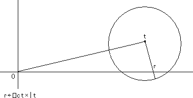
More precisely, it is the union of two circular regions: The smaller is centered on t with radius r . The larger derives as follows. A point u on the boundary with magnitude ≥ |t satisfies (|u-t)=⎕ct×|u . That is, the ratio between |u-t and |u is ⎕ct , a constant; therefore, that boundary is a circle of Apollonius with foci t and the origin. The larger circle circumscribes the two points on the smaller circle with magnitude |t and the point with magnitude (|t)÷1-⎕ct collinear with t and the origin. (A more precise diagram than the one above can be found in Appendix A0.)

The union of two circles (or even a circle) is inconvenient to deal with computationally. For present purposes it is good enough to work with a square that contains the region, “good enough” in the sense that even though numbers outside the region will be hashed to the same index, such numbers will be rejected when they are tested for tolerant equality. We choose as the delta (half the length of a side of the square) ⎕ct × √2 × the larger of the magnitudes of the real and imaginary parts of t . This choice avoids the problem and expense of computing the magnitude of t , requisite for a tighter fitting square.


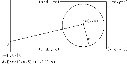
   delta←{⍺←⎕ct ⋄ ⍺×(2*0.5)×⌈/|9 11○⍵}

   delta 3j4
5.656854249E¯14
   delta 3e6j4
4.242640687E¯8
   delta 3j4e6
5.656854249E¯8

Like the real case, the leading bits of the four corners are representative of those of points in the square. However, unlike the real case, the number of leading bits will depend on ⎕ct and t and (in general) are different for the real and imaginary parts.

   hexf 3 4
4008000000000000 4010000000000000
   hexf 3 4+○1e¯14
4008000000000047 4010000000000023

   hexf 3 1e¯20
4008000000000000 3BC79CA10C924223
   hexf 3, ○¯1e¯21
4008000000000000 BBADABE7AA9FDCC0

The first example shows that if the limbs (the real and imaginary parts) are similar in length, then the numbers in the region can have many common leading bits in both limbs. The second example shows that if one limb is much longer than the other, then two tolerantly equal numbers can have completely different bits in their shorter limbs.

For a complex number t , the number of leading bits for the longer limb is computed as before, a function of ⎕ct alone (function hashmask). The number of leading bits for the shorter limb s with a delta of d is the length of the common prefix for s and s+d or for s and s-d , whichever is longer (function hashmask2).

A hashing algorithm for x⍳y for complex x and y :

0.  Compute a mask based on ⎕ct (function hashmask).
1.  Initialize a hash table h of size prime q larger than 2×⍴x .
2.  For each element i⌷x , compute d←delta i⌷x and m2←s hashmask2 d where s is the length of the shorter limb, then mask out the trailing bits separately for the real and imaginary parts, then compute a hash index, then insert into the hash table at that index. Collisions of elements that are not exactly equal are resolved by inserting into the next hash table entry, wrapping back to the front as necessary. Exactly equal elements are inserted just once.
3.  For each element i⌷y , compute d←delta i⌷y and m2←s hashmask2 d where s is the length of the shorter limb, then for each of the “four corners”
  (i⌷y) + d ×  1j1
  (i⌷y) + d ×  1j¯1
  (i⌷y) + d × ¯1j1
  (i⌷y) + d × ¯1j¯1
mask out the trailing bits separately for the real and imaginary parts, then compute a hash index, then look in the hash table starting at that index, using tolerant equality.

The hash index for a 128-bit masked complex number t is q|(p0×t0)+(p1×t1)+(p2×t2)+(p3×t3) , where t0 t1 t2 t3 are the parts of t cast as 32-bit integers, p0 p1 p2 p3 are 32-bit primes, and q is the size of the hash table. (See function zhashfn.) In the C implementation, the expression ignores (indeed exploits) integer overflow.

The algorithm is modelled in APL as ziota , written as a “tradfn” to facilitate translation into C.

   x←*0j1×1+(0.25×⎕ct)×?199⍴223
   y←*0j1×1+(0.25×⎕ct)×?307⍴239
   (x iota y)≡x ziota y
1

3. Implementation

The algorithms modelled by diota and ziota have been implemented in C in Dyalog v. 13.0. The same algorithms underlie the implementation of x∊y x~y x∩y x∪y ∪x . The implementation has additional optimizations for ⎕ct←0 and for x⍳x and ∪x where the initial hashing of x (step 2) is merged into the main loop (step 3). The hash table is retained for reuse in f←x∘⍳ and in x∘⍳¨ (also ∊∘y , etc.).
 

4. Tests

assert p is a monad which does nothing if ~0∊p and signals assertion failure if 0∊p . For example:

   x←1000 rand 0.5
   assert (x⍳x)≡x iota x

   assert 3 = 3×1+2×⎕ct
assertion failure
   assert 3=3×1+2×⎕ct
  ∧

The test suites use assert extensively. A test function returns a 1 if it runs successfully, or suspends with an assertion failure at the first point of failure. Four main functions are included (see Appendix A2):

   test_iotaD           ⍝ x⍳y for real x and y
1
   test_iotaD_retained  ⍝ f←x∘⍳ and x∘⍳¨ for real x
1
   test_iotaZ           ⍝ x⍳y for complex x and y
1
   test_iotaZ_retained  ⍝ f←x∘⍳ and x∘⍳¨ for complex x
1

5. Timings

The following table compares the timings in Dyalog v13.0 vs. v12.1.

{x y←⍵ ⍵ rand¨0.5 ⋄ 5 timer'x⍳y'}¨1e6×1 2 4 8
{x  ←⍵   rand 0.5 ⋄ 5 timer'x⍳x'}¨1e6×1 2 4 8
       Real x⍳y       Real x⍳x      
n  v13.0   v12.1   Ratio  v13.0   v12.1   Ratio 
1e6  0.5812  2.3438 4.03  0.3282  2.1282 6.48 
2e6  1.2438  5.2124 4.19  0.6906  5.0874 7.37 
4e6  2.2938  11.1250 4.85  1.3438  11.1844 8.32 
8e6  4.9750  25.9906 5.22  2.9562  24.8844 8.42 

The following table presents timings done only in Dyalog v13.0 as they are impossible or impractical in v12.1.

{x y←⍵ ⍵ rand¨0j1 ⋄ 5 timer'x⍳y'}¨1e6×1 2 4 8
{x  ←⍵   rand 0j1 ⋄ 5 timer'x⍳x'}¨1e6×1 2 4 8
{x y←monster¨⍵ ⍵  ⋄ 5 timer'x⍳y'}¨1e6×1 2 4 8
{x  ←monster ⍵    ⋄ 5 timer'x⍳x'}¨1e6×1 2 4 8
       Complex      Monster
n  x⍳y   x⍳x   x⍳y   x⍳x 
1e6  1.6500  0.9532  1.8032  1.6750
2e6  3.2750  2.1436  3.5032  3.2314
4e6  5.1468  3.6906  6.8906  6.8562
8e6  9.7032  7.2250  13.3812  13.3436

References

0.  ISO/IEC, Programming Language Extended APL, ISO/IEC 13751:2001(E), 2001-02-01; Section 5.2.5, Tolerantly-Equal, page 19.
1.  Bernecky, Robert, e-mail, 2010-05-11 05:04.
2.  Streeter, Geoff, e-mail, 2010-05-13 00:25.
3.  Koss, Steven L., Tolerant Hash Functions, Minnowbrook, 1985-10.
4.  Knuth, Donald E., The Art of Computer Programming, Volume 3, Searching and Sorting, Addison-Wesley, 1973; Section 6.4.

Appendices

A0. Region of Tolerant Equality

The region of numbers tolerantly equal to a complex number t is a near-circle with radius r←⎕ct×|t .


More precisely, it is the union of two circular regions: The smaller (in black) is centered on t with radius r . The larger derives as follows. A point u on the boundary with magnitude ≥ |t satisfies (|u-t)=⎕ct×|u . That is, the ratio between |u-t and |u is ⎕ct , a constant; therefore, that boundary is a circle of Apollonius with foci t and the origin. The larger circle (in red) circumscribes the two points p and q on the smaller circle with magnitude |t (in green) and the point s with magnitude (|t)÷1-⎕ct collinear with t and the origin.

         
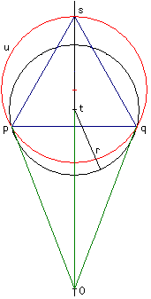
r←⎕ct×|t

(|u-t) = ⎕ct×|u
(|p)   = |t
(|q)   = |t
(|s)   = (|t)÷1-⎕ct

If t is real, the region simplifies to the closed interval with endpoints t×1-⎕ct and t÷1-⎕ct .


A1. Models

bfh       ← {((¯1↓⍴⍵),4ׯ1↑⍴⍵)⍴(¯1⌽⍳1+⍴⍴⍵)⍉(4⍴2)⊤'0123456789ABCDEF'⍳⍵}

binary    ← {((⍴⍵),64)⍴⍉(4⍴2)⊤'0123456789ABCDEF'⍳,0 1↓((×/⍴⍵),17)⍴' ',hexf ⍵}

dhashfn   ← {⍺|2294967341 17 hfn ⍵}

decf        ⍝ from dfns workspace

delta     ← {⍺←⎕ct ⋄ ⍺×(2*0.5)×⌈/|9 11○⍵}

∇ z←{qct}fourcorners xy;b;bx;by;d;m;px;py;t
 ⍝ the 4 corners of a square that contains the circle of equality
 ⍝ e.g.   fourcorners 10 4   or   1e¯10 fourcorners (*1),1e¯12
 ⍝ xy:  2-element vector of the real and imaginary parts
 ⍝ qct: comparison tolerance (default: ⎕ct)
  ⍎(0=⎕nc 'qct')/'qct←⎕ct'
  m←⌈/|xy                      ⍝ the larger magnitude
  d←qct×m×2*0.5                ⍝ displacement to corner
  t←(4 2⍴xy)+d×1-2×⍉2 2⊤⍳4     ⍝ the 4 corners
  b←bfh 0 1↓8 17⍴' ',hexf t    ⍝ t in binary
  bx←(8⍴1 0)⌿b                 ⍝ real      parts in binary
  by←(8⍴0 1)⌿b                 ⍝ imaginary parts in binary
  b←bfh 0 1↓2 17⍴' ',hexf xy   ⍝ original numbers in binary
  px←hfb∨⌿∧\bx=b[4⍴0;]         ⍝ mask for real      parts
  py←hfb∨⌿∧\by=b[4⍴1;]         ⍝ mask for imaginary parts
  z←(6 5⍴'orig mask c0   c1   c2   c3   '),(hexf xy)⍪(px,' ',py)⍪hexf t
∇

hashmask  ← {∧\∧⌿t[0 0;]=1 0↓t←binary ⍺×1,m,÷m←1-⍵}

hashmask2 ← {64↑1⍴⍨(16≤n)×8×⌊8÷⍨n←+/∨⌿∧\t[0 0;]=1 0↓t←binary ⍺,(⍺-⍵),⍺+⍵}

hexf        ⍝ from dfns workspace 

hfb       ← {'0123456789ABCDEF'[2⊥(1⌽⍳1+⍴⍴⍵)⍉((¯1↓⍴⍵),((¯1↑⍴⍵)÷4),4)⍴⍵]}

hfn       ← {
 ⍝ subfunction of dhashfn and zhashfn
 ⍝ ⍺: two 32-bit primes
 ⍝ ⍵: 64-bit integer as a 64-element boolean vector
    p0←(2⍴65536)⊤⍺[0]                        ⍝ p0 as two 16-bit numbers
    p1←(2⍴65536)⊤⍺[1]                        ⍝ p1 as two 16-bit numbers
    h←2⊥⍉4 16⍴⍵                              ⍝ ⍵ as 4 16-bit numbers
    t←+⌿0 ¯1⌽2 3↑p0∘.×2↑h                    ⍝ now implement (p0×y0)+(p1×y1)
    t←¯2↑t++⌿0 ¯1⌽2 3↑p1∘.×2↓h
    65536⊥{1↓(0,65536|⍵)+(⌊⍵÷65536),0}⍣≡t    ⍝ propagate carries
}

iota      ← {(0⌷⍴⍺)-+/∨\⍵∘.=⍺}

intv      ← {⍺←⎕ct ⋄ ⍵×(1-⍺),1,÷1-⍺}

j         ← {⍺←0 ⋄ ⍺+0j1×⍵}

monster   ← {1+(0.0001×⎕ct)×?⍵⍴100000}

permute   ← {⍵[?⍨⍴⍵]}

Primes    ← 1031 2053 4099 8209 16411 32771 65537 131101 262147 524309 
                1048583 2097169 4194319 8388617 16777259 33554467 67108879 
                134217757 268435459 536870923
            ⍝ next prime >2*k, k≥10

rand      ← {
 ⍝ generate random data with shape ⍺ and range ⍵
     ⍵=0.5   : 256÷⍨¯200000+?⍺⍴500000
     ⍵=0j1   : 1 0j1+.×8÷⍨¯500+?(2,⍺)⍴1000
     ⍵=⌊/⍳0  : ⍺⍴permute,(1 ¯1×⍵)∘.×1-⎕ct×16÷⍨?⍺⍴113
     1e¯99>⍵ : ⍺⍴permute,(1 ¯1×⍵)∘.×1+⎕ct×16÷⍨?⍺⍴113  ⍝ ⍵ = decf 15 1/'01'
     t←⎕DR y←((2≠⍵)×⌊⍵÷¯2)+?⍺⍴⍵ ⋄ y
}


∇ z9←{x9}timer y9;c9;i9
 ⍝ the average seconds required to execute expression y9 x9 times
  ⍎(0=⎕nc 'x9')/'x9←1'
  c9←⎕ai
  :For i9 :In ⍳x9
      ⍎''
  :EndFor
  c9←⎕ai-c9
  z9←⎕ai
  :For i9 :In ⍳x9
      {}⍎y9
  :EndFor
  z9←⎕ai-z9
  z9←(z9-c9)[1+⎕io]÷1000×x9
∇

∇ z←q zhashfn x;b;m;p0;p1;p2;p3;q;s;t
 ⍝ hash function on complex number x, using modulus q
 ⍝ x: 2 64 boolean matrix of the real and imaginary parts of a complex number
  s←2294967341 17 hfn x[0;]  ⍝ hash real part
  t←2394967363 43 hfn x[1;]  ⍝ hash imaginary part
  z←q|(2*32)|s+t
∇

∇ z←x diota y;h;hj;i;j;k;m0;m1;mask;ne0;q;yi;yy
 ⍝ model of x⍳y where x and y are 64-bit floating point numbers and ⎕ct>0

  q←Primes[(Primes>2×⍴x)⍳1]                 ⍝ size of hash table, a prime >2×⍴x
  h←q⍴¯1                                    ⍝ hash table; ¯1 means "free"
  m1←÷m0←1-⎕ct                              ⍝ upper & lower multipliers
  mask←(○1)hashmask ⎕ct                     ⍝ bits in a 64-bit number to hash
  ne0←{⎕ct←0 ⋄ ⍺≠⍵}                         ⍝ exact not-equal

  :For i :In ⍳⍴x                            ⍝ hash x
      j←q dhashfn mask∧binary x[i]          ⍝ index into hash table
      :While (0≤h[j])∧x[i] ne0 x[0⌈h[j]]    ⍝ don't table exact duplicates
          j←q|1+j                           ⍝ the next hash table entry
      :EndWhile
      ⍎(0>h[j])/'h[j]←i'                    ⍝ new hash continuation
  :EndFor

  z←(⍴y)⍴¯1
  :For i :In ⍳⍴y                            ⍝ main loop
      k←⍴x                                  ⍝ index of y[i] as far as we now know
      yi←{mask∧binary ⍵}¨y[i]×m0,m1         ⍝ masked variants
      :For yy :In ∪yi                       ⍝ do for each unique variant
          j←q dhashfn yy                    ⍝ where to start looking in hash table
          :While 0≤hj←h[j]                  ⍝ loop until no more hash continuations
              ⍎((k>hj)∧y[i]=x[hj])/'k←hj'   ⍝ look for tolerant match with smaller index
              j←q|1+j                       ⍝ do next hash continuation
          :EndWhile
      :EndFor
      z[i]←k
  :EndFor
∇

∇ z←x ziota y;c;d;diag;h;hj;i;j;k;mask;msk;ne0;p;q;t;yi;yy
 ⍝ model of x⍳y where x and y are complex numbers and ⎕ct>0

  q←Primes[(Primes>2×⍴x)⍳1]                 ⍝ size of hash table, a prime >2×⍴x
  h←q⍴¯1                                    ⍝ hash table; ¯1 means "free"
  diag←⎕ct×2*0.5                            ⍝ relative displacement to a corner
  mask←(○1)hashmask ⎕ct                     ⍝ bits in a 64-bit number to hash
  ne0←{⎕ct←0 ⋄ ⍺≠⍵}                         ⍝ exact not-equal

  :For i :In ⍳⍴x                            ⍝ hash x
      t←9 11○x[i]                           ⍝ real and imaginary parts
      msk←(⌊/|t)hashmask2 diag×⌈/|t         ⍝ mask for shorter limb
      c←(binary t)∧(</|t)⊖mask,[¯0.5]msk
      j←q zhashfn c                         ⍝ index into hash table
      :While (0≤h[j])∧x[i] ne0 x[0⌈h[j]]    ⍝ don't table exact duplicates
          j←q|1+j                           ⍝ the next hash table entry
      :EndWhile
      ⍎(0>h[j])/'h[j]←i'                    ⍝ new hash continuation
  :EndFor

  z←(⍴y)⍴¯1
  :For i :In ⍳⍴y                            ⍝ main loop
      k←⍴x                                  ⍝ index of y[i] as far as we now know
      t←9 11○y[i]                           ⍝ real and imaginary parts
      d←diag×⌈/|t                           ⍝ absolute displacement to a corner
      msk←(⌊/|t)hashmask2 d                 ⍝ mask for shorter limb
      yi←{binary t+d×⍵}¨,∘.,⍨1 ¯1           ⍝ 4 corners of square containing the region of equality
      yi←yi∧¨⊂(</|t)⊖mask,[¯0.5]msk         ⍝ masked variants; see also function "fourcorners"
      :For yy :In ∪yi                       ⍝ do for each unique variant
          j←q zhashfn yy                    ⍝ where to start looking in hash table
          :While 0≤hj←h[j]                  ⍝ loop until no more hash continuations
              ⍎((k>hj)∧y[i]=x[hj])/'k←hj'   ⍝ look for tolerant match with smaller index
              j←q|1+j                       ⍝ do next hash continuation 
          :EndWhile
      :EndFor
      z[i]←k
  :EndFor
∇

A2. Tests

∇ assert x
  'assertion failure' ⎕signal (0∊x)⍴11
∇

Domains ← 2 256 65536 2000000000 0.5 0j1

∇ z←test_iotaD;b;e;i;j;m;x;y
 ⍝ tests on dyadic iota with 64-bit float left argument

  x←256÷⍨i←¯4500+?10000⍴9000
  y←256÷⍨j←¯4500+?10000⍴10000
  assert(x⍳x)≡i⍳i
  assert(x⍳y)≡i⍳j

  x←1+⎕ct×?200⍴150
  y←1+⎕ct×?300⍴250
  assert(x⍳x)≡x iota x
  assert(x⍳y)≡x iota y

  x←1+(0.25×⎕ct)×?200⍴851
  y←1+(0.25×⎕ct)×?300⍴951
  assert(x⍳x)≡x iota x
  assert(x⍳y)≡x iota y

  assert b←((⍳20),1000+⍳8)∘.{(1+x⍳y)≡((○1),x←⍺ rand ⍵)⍳y←⍺ rand ⍵}Domains
  assert b←((⍳20),1000+⍳8)∘.{x←⍺ rand ⍵ ⋄ (⍺,x⍳y)≡x⍳(○1),y←⍺ rand ⍵}Domains

  m←⌊/⍳0  ⍝ m: largest positive number
  x←89 rand m
  y←97 rand m
  assert(x⍳x)≡x iota x
  assert(y⍳y)≡y iota y
  assert(x⍳y)≡x iota y

  e←decf 15 1/'01'  ⍝ e: smallest positive number
  x←89 rand e
  y←97 rand e
  assert(x⍳x)≡x iota x
  assert(y⍳y)≡y iota y
  assert(x⍳y)≡x iota y

  z←1
∇

∇ z←test_iotaD_retained;b;g;i;j;n;qct;t;x;y
 ⍝ tests on dyadic iota with 64-bit float left or right argument

  qct←1.5×⎕ct

  x←256÷⍨i←¯4500+?10000⍴9000
  y←256÷⍨j←¯4500+?10000⍴10000
  g←x∘⍳
  assert(g x)≡i⍳i
  assert(g y)≡i⍳j
  assert b←((⍳20),1000+⍳8)∘.{(g y)≡x⍳y←⍺ rand ⍵}Domains
  assert b←((⍳20),1000+⍳8)∘.{⎕ct←qct ⋄ (g y)≡x⍳y←⍺ rand ⍵}Domains
  assert(b⊂x⍳y)≡¨x∘⍳¨(b←1,0=1↓?(⍴y)⍴1000)⊂y
  assert{⎕ct←⍵ ⋄ (g y)≡x⍳y}¨⎕ct×0.25×1+⍳6

  x←1+⎕ct×?200⍴150
  y←1+⎕ct×?300⍴250
  g←x∘⍳
  assert(g x)≡x iota x
  assert(g y)≡x iota y
  assert b←((⍳20),1000+⍳8)∘.{(g y)≡x⍳y←⍺ rand ⍵}Domains
  assert b←((⍳20),1000+⍳8)∘.{⎕ct←qct ⋄ (g y)≡x⍳y←⍺ rand ⍵}Domains
  assert(b⊂x⍳y)≡¨x∘⍳¨(b←1,0=1↓?(⍴y)⍴50)⊂y
  assert{⎕ct←⍵ ⋄ (g y)≡x⍳y}¨⎕ct×0.25×1+⍳6

  x←1+(0.25×⎕ct)×?200⍴851
  y←1+(0.25×⎕ct)×?300⍴951
  g←x∘⍳
  assert(g x)≡x iota x
  assert(g y)≡x iota y
  assert b←((⍳20),1000+⍳8)∘.{(g y)≡x⍳y←⍺ rand ⍵}Domains
  assert b←((⍳20),1000+⍳8)∘.{⎕ct←qct ⋄ (g y)≡x⍳y←⍺ rand ⍵}Domains
  assert(b⊂x⍳y)≡¨x∘⍳¨(b←1,0=1↓?(⍴y)⍴50)⊂y
  assert{⎕ct←⍵ ⋄ (g y)≡x⍳y}¨⎕ct×0.25×1+⍳6

  n←(⍳20),1000+⍳8
  assert b←n∘.{x←⍺ rand ⍵ ⋄ g←x∘⍳ ⋄ t←g 4 ⋄ (g(○1),y)≡⍺,x⍳y←⍺ rand ⍵}Domains
  assert b←n∘.{x←⍺ rand ⍵ ⋄ g←((○1),x)∘⍳ ⋄ t←g 4 ⋄ (g y)≡1+x⍳y←⍺ rand ⍵}Domains

  x←0.01ׯ200000+?1000000⍴500000
  y←0.01ׯ200000+?100⍴500000
  g←x∘⍳
  assert(g y)≡x⍳y
  assert 0.1>t←(5 timer'g y')÷5 timer'x⍳y'

  z←1
∇

∇ z←test_iotaZ;b;e;f;m;p;q;x;y
 ⍝ tests on dyadic iota with complex left argument

  x←1 0j1+.×16÷⍨p←¯45+?2 10000⍴90
  y←1 0j1+.×16÷⍨q←¯45+?2 10000⍴100
  assert(x⍳x)≡p⍳p←100⊥p
  assert(x⍳y)≡p⍳q←100⊥q

  x←1 0j1+.×17÷⍨p←¯45+?2 10000⍴90
  y←1 0j1+.×17÷⍨q←¯45+?2 10000⍴100
  assert(x⍳x)≡p⍳p←100⊥p
  assert(x⍳y)≡p⍳q←100⊥q

  x←1 0j1+.×1+⎕ct×?2 199⍴53
  y←1 0j1+.×1+⎕ct×?2 307⍴59
  assert(x⍳x)≡x iota x
  assert(x⍳y)≡x iota y

  x←1 0j1+.×1+(0.25×⎕ct)×?2 199⍴223
  y←1 0j1+.×1+(0.25×⎕ct)×?2 307⍴239
  assert(x⍳x)≡x iota x
  assert(x⍳y)≡x iota y

  x←*j 1+(0.25×⎕ct)×?199⍴223
  y←*j 1+(0.25×⎕ct)×?307⍴239
  assert(x⍳x)≡x iota x
  assert(x⍳y)≡x iota y

  x←(0.5ׯ12+?199⍴23)j ⎕ct×?199⍴30
  y←(0.5ׯ12+?307⍴23)j ⎕ct×?307⍴30
  assert(x⍳x)≡x iota x
  assert(x⍳y)≡x iota y

  x←(0.5ׯ12+?199⍴23)j⍨⎕ct×?199⍴30
  y←(0.5ׯ12+?307⍴23)j⍨⎕ct×?307⍴30
  assert(x⍳x)≡x iota x
  assert(x⍳y)≡x iota y

  x←((⎕ct×?120⍴30),0.5ׯ12+?79⍴23)[?⍨199]j((⎕ct×?120⍴30),0.5ׯ12+?79⍴23)[?⍨199]
  y←((⎕ct×?209⍴30),0.5ׯ12+?98⍴23)[?⍨307]j((⎕ct×?209⍴30),0.5ׯ12+?98⍴23)[?⍨307]
  assert(x⍳x)≡x iota x
  assert(x⍳y)≡x iota y

  assert b←((⍳20),1000+⍳20)∘.{(1+x⍳y)≡((3 j○1),x←⍺ rand ⍵)⍳y←⍺ rand ⍵}Domains
  assert b←((⍳20),1000+⍳20)∘.{(⍺,x⍳y)≡(x←⍺ rand ⍵)⍳(3 j○1),y←⍺ rand ⍵}Domains

  z←1
∇

∇ z←test_iotaZ_retained;b;g;i;k;n;qct;t;x;y
 ⍝ tests on dyadic iota with complex arguments

  qct←1.5×⎕ct

  x←1 0j1+.×256÷⍨i←¯250+?2 10000⍴500
  y←1 0j1+.×256÷⍨k←¯250+?2 10000⍴500
  g←x∘⍳
  assert(g x)≡i⍳i←500⊥i
  assert(g y)≡i⍳k←500⊥k
  assert b←((⍳20),1000+⍳8)∘.{(g y)≡x⍳y←⍺ rand ⍵}Domains
  assert b←((⍳20),1000+⍳8)∘.{⎕ct←qct ⋄ (g y)≡x⍳y←⍺ rand ⍵}Domains
  assert(b⊂x⍳y)≡¨x∘⍳¨(b←1,0=1↓?(⍴y)⍴1000)⊂y
  assert{⎕ct←⍵ ⋄ (g y)≡x⍳y}¨⎕ct×0.25×1+⍳6

  x←*j 1+⎕ct×?200⍴150
  y←*j 1+⎕ct×?300⍴250
  g←x∘⍳
  assert(g x)≡x iota x
  assert(g y)≡x iota y
  assert b←((⍳20),1000+⍳8)∘.{(g y)≡x⍳y←⍺ rand ⍵}Domains
  assert b←((⍳20),1000+⍳8)∘.{⎕ct←qct ⋄ (g y)≡x⍳y←⍺ rand ⍵}Domains
  assert(b⊂x⍳y)≡¨x∘⍳¨(b←1,0=1↓?(⍴y)⍴50)⊂y
  assert{⎕ct←⍵ ⋄ (g y)≡x⍳y}¨⎕ct×0.25×1+⍳6

  x←*j 1+(0.25×⎕ct)×?200⍴851
  y←*j 1+(0.25×⎕ct)×?300⍴951
  g←x∘⍳
  assert(g x)≡x iota x
  assert(g y)≡x iota y
  assert b←((⍳20),1000+⍳8)∘.{(g y)≡x⍳y←⍺ rand ⍵}Domains
  assert b←((⍳20),1000+⍳8)∘.{⎕ct←qct ⋄ (g y)≡x⍳y←⍺ rand ⍵}Domains
  assert(b⊂x⍳y)≡¨x∘⍳¨(b←1,0=1↓?(⍴y)⍴50)⊂y
  assert{⎕ct←⍵ ⋄ (g y)≡x⍳y}¨⎕ct×0.25×1+⍳6

  x←(0.5ׯ12+?199⍴23)j ⎕ct×?199⍴30
  y←(0.5ׯ12+?307⍴23)j ⎕ct×?307⍴30
  g←x∘⍳
  assert(g x)≡x iota x
  assert(g y)≡x iota y
  assert b←((⍳20),1000+⍳8)∘.{(g y)≡x⍳y←⍺ rand ⍵}Domains
  assert b←((⍳20),1000+⍳8)∘.{⎕ct←qct ⋄ (g y)≡x⍳y←⍺ rand ⍵}Domains
  assert(b⊂x⍳y)≡¨x∘⍳¨(b←1,0=1↓?(⍴y)⍴50)⊂y
  assert{⎕ct←⍵ ⋄ (g y)≡x⍳y}¨⎕ct×0.25×1+⍳6

  n←(⍳20),1000+⍳8
  assert b←n∘.{x←⍺ rand ⍵ ⋄ g←x∘⍳ ⋄ t←g 4 ⋄ (g(3 j○1),y)≡⍺,x⍳y←⍺ rand ⍵}Domains
  assert b←n∘.{x←⍺ rand ⍵ ⋄ g←((3 j○1),x)∘⍳ ⋄ t←g 4 ⋄ (g y)≡1+x⍳y←⍺ rand ⍵}Domains

  x←0.01 0j0.01+.ׯ450+?2 500000⍴900
  y←0.01 0j0.01+.ׯ450+?2 100⍴900
  g←x∘⍳
  assert(g y)≡x⍳y
  assert 0.1>t←(5 timer'g y')÷5 timer'x⍳y'

  z←1
∇


This text requires the APL385 Unicode font, which can be downloaded from http://www.vector.org.uk/resource/apl385.ttf . To resolve (or at least explain) problems with displaying APL characters see http://www.vector.org.uk/archive/display.htm .

original writing:  2010-05-13 20:15
last updated:2010-08-12 09:05