

By: Stefan Kruger
Stefan works for IBM making databases. He tries to learn at least one new programming language a year, and a few years ago he got hooked on APL and participated in the competition. This is his perspective on some solutions that the judges picked out – call it the “Judges’ Pick”, if you like; smart, novel, or otherwise noteworthy solutions that can serve as an inspiration.
Congratulations to all the winners of the 2021 APL Problem Solving Competition (you can learn more about the phase 2 winners in this article) and well done to Dzintars Klušs who won the Grand Prize. At the recent Dyalog ’21 user meeting, we got to enjoy the runner-up, Victor Ogunlokun, walking us through his solutions live.
In this post I’ll go through some great solutions that were submitted (and some that weren’t submitted) to the Phase I problems so that we can all marvel in the ingenuity and perhaps learn a thing or two. If you’re feeling inspired by the end, go ahead and participate in this year’s round which just launched.
If you’re new to the APL Problem Solving Competition, Phase I problems tend to be short and the expectation is that solutions will be “one-liners” (dfns). However, although it might seem like it from some of the solutions here, this isn’t a code golf competition! Solutions are judged holistically: do they solve the problem, are they efficient, and are they clear? Even though a few test cases are given, there is no guarantee that your solution is correct just because it works for the example data. The judging process involves running the code on many hidden test cases too. Crucially, just because your code is accepted, it doesn’t necessarily mean that you’ll get full marks.
As with my blog post that reviewed the 2020 Phase II solutions, I’ve included a more in-depth examination of one or two problems.
Problem 1: Are You a Bacteria?
Something from the excellent Project Rosalind problem collection, the task is to compute the combined percentage of guanine (G) and cytosine (C) in a given DNA-string.
Efficiency can vary a lot, depending on whether summation or multiplication (or even division!) is performed first. Some solutions were also leading-axis oriented.
Here’s my solution:
      {100×(+⌿⍵∊'CG')÷≢⍵} 'ACGTACGTACGTACGT'
50
which several competitors made more tacit with:
      {100×(+⌿÷≢)⍵∊'GC'} 'ACGTACGTACGTACGT'
50
or even went further:
      (100×≢÷⍨1⊥∊∘'GC') 'ACGTACGTACGTACGT'
50
If you’re unfamiliar with the 1⊥ trick, it’s a way of summing a vector:
      1⊥6 3 9 8 12 62
100
It’s perhaps not immediately obvious why this should work. Here’s one explanation. Assume we want to sum the vector 1 0 2 0 0. We can do this in a very convoluted way by using a sum inner product with a vector of exponentials: [14, 13, 12, 11, 10]:
      (1*4 3 2 1 0)+.×1 0 2 0 0
3
If we expand the exponentials to the left we get a vector of 1s. We can then break apart the inner product by turning +. to a +⌿ to the left:
      +⌿1 1 1 1 1×1 0 2 0 0
3
This is the textbook definition of 1⊥! Look:
      1⊥1 0 2 0 0
3
which, to be clear, is just the sum-reduce-first:
      +⌿1 0 2 0 0
3
Using 1⊥ to sum has two advantages over the more obvious formulation +⌿. Firstly, it’s easier to use in tacit formulations as it doesn’t require an operator, and secondly, it’s usually faster. The reasons for it being quicker is somewhat beyond the scope of this post, but it’s to do with 1⊥ making no guarantees about the ordering of operations, meaning that the interpreter is free to vectorise more efficiently.
Problem 2: Index-Of Modified
This problem wanted us to write a function that behaves like the APL Index Of function R←X⍳Y except that it should return 0 for elements of Y not found in X.
I wrote:
      p2 ← {0@((≢⍺)∘<)⊢⍺⍳⍵}
      2 3 p2 ⍳5
0 1 2 0 0
which is basically saying “change all instances of numbers greater than the length of the argument to zero”, which is how X⍳Y presents values that are not found.
Some very different solutions were submitted, for example:
      p2 ← ⍳|⍨1+≢⍤⊣
      2 3 p2 ⍳5
0 1 2 0 0
which is simply:
      p2 ← {(1+≢⍺)|⍺⍳⍵} ⍝ dfn of the above
      2 3 p2 ⍳5
0 1 2 0 0
Another option would have been to multiply ⍺⍳⍵ with ≢⍺, although no-one submitted exactly this:
      p2 ← ≢⍤⊣(≥×⊢)⍳
      2 3 p2 ⍳5
0 1 2 0 0
which could have been written explicitly as:
      p2 ← {m×(≢⍺)≥m←⍺⍳⍵} ⍝ dfn of the above
      2 3 p2 ⍳5
0 1 2 0 0
Problem 3: Multiplicity
Write a function that:
- has a right argument
Ywhich is an integer vector or scalar - has a left argument
Xwhich is also an integer vector or scalar - finds which elements of
Yare multiples of each element ofXand returns them as a vector (in the order ofX) of vectors (in the order ofY).
Some test data was provided:
      X ← 2 4 7 3 9
      Y ← 5 7 8 1 12 10 20 16 11 4 2 15 3 18 14 19 13 9 17 6
I wrote something that, in retrospect, looks somewhat clumsy:
      p3 ← {⍵∘{⍵/⍺}¨↓0=⍺∘.|,⍵}
      X p3 Y
┌─────────────────────────┬────────────┬────┬──────────────┬────┐
│8 12 10 20 16 4 2 18 14 6│8 12 20 16 4│7 14│12 15 3 18 9 6│18 9│
└─────────────────────────┴────────────┴────┴──────────────┴────┘
which can be expressed more compactly as:
      p3 ← {/∘⍵¨↓0=⍺∘.|⍥,⍵}
      X p3 Y
┌─────────────────────────┬────────────┬────┬──────────────┬────┐
│8 12 10 20 16 4 2 18 14 6│8 12 20 16 4│7 14│12 15 3 18 9 6│18 9│
└─────────────────────────┴────────────┴────┴──────────────┴────┘
or:
      X (⊢⊂⍤/⍤1⍨0=∘.|⍥,) Y
┌─────────────────────────┬────────────┬────┬──────────────┬────┐
│8 12 10 20 16 4 2 18 14 6│8 12 20 16 4│7 14│12 15 3 18 9 6│18 9│
└─────────────────────────┴────────────┴────┴──────────────┴────┘
although no-one actually submitted that, to everyone’s credit.
Problem 4: Square Peg, Round Hole
Write a function that:
- takes a right argument which is an array of positive numbers representing circle diameters
- returns a numeric array of the same shape as the right argument representing the difference between the areas of the circles and the areas of the largest squares that can be inscribed within each circle.
I had to read that many times before it sank in. The key to achieve something snappy is to really work through the maths until it is as compact as possible, which, if you’re anything like me, you didn’t bother to do.
My attempt was:
p4 ← {(○2*⍨⍵÷2)-2÷⍨⍵*2}
but there are much neater solutions if you did your homework. Here’s one that no-one found:
p4 ← (○-+⍨)4÷⍨×⍨
and a nice explicit version:
p4 ← {⍵×⍵×0.5-⍨○÷4}
which can be derived from this simplified mathematical expression, suggested by Rodrigo:
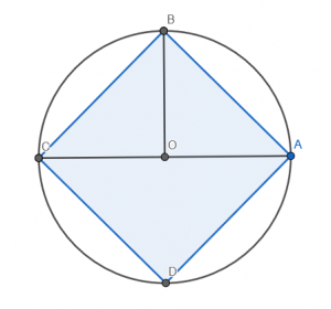
Explanation: The area of the circle is ○r*2, which is ○(⍵÷2)*2, in turn equivalent to ⍵×⍵×○÷4. The area of the square [ABCD] is twice the area of the triangle [ABC]. Given that the area of the triangle is 0.5×⍵×⍵÷2, the area of the square becomes 0.5×⍵×⍵. Putting both together, we get (⍵×⍵×○÷4)-⍵×⍵×0.5, the same as ⍵×⍵×(○÷4)-0.5, which is ⍵×⍵×0.5-⍨○÷4.
Problem 5: Rect-ify
For this problem, we were asked to plant a number of trees in a rectangular pattern with complete rows and columns, meaning all rows have the same number of trees. That rectangular pattern also needed to be as “square as possible”, meaning there is a minimal difference between the number of rows and columns in the pattern.
Here’s a smart solution, based on the observation that the “most square” choice must have one factor being the largest factor less than or equal to the square root:
p5 ← {N,⍵÷1⌈N←⌈/0,⍵∨⍳⌊⍵*÷2}
This solution works well on large numbers of trees, too:
      p5 98776512304
280888 351658
Someone even offered up a recursive solution:
p5rec ← {⍵=0:2⍴0 ⋄ ⍵ {0=⍵|⍺: ⍵,⍺÷⍵ ⋄ ⍺∇⍵-1} ⌊⍵*÷2}
So is one solution better than the other? Well, they both work correctly, but one is a lot faster than the other. Do you want to guess which was faster before we test it?
      'cmpx'⎕CY'dfns'
      cmpx 'p5 98776512304' 'p5rec 98776512304'
  p5 98776512304    → 8.7E¯2 |   0% ⎕⎕⎕⎕⎕⎕⎕⎕⎕⎕⎕⎕⎕⎕⎕⎕⎕⎕⎕⎕⎕⎕⎕⎕⎕⎕⎕⎕⎕⎕⎕⎕⎕⎕⎕⎕⎕⎕⎕⎕
  p5rec 98776512304 → 6.1E¯3 | -94% ⎕⎕⎕
Surprised? I was! So, what is going on here? The non-recursive solution relies on a rather crude way to find the factors, which is a fairly large number to factorise even if it only needs to go up to the square root. The recursive version just tries each number in turn, up to the square root.
Can we be even smarter? This version was offered up by APL Orchard regular @rak1507:
p5rak1507 ← {a,⍵÷1⌈a←⊃⌽⍸0=⍵|⍨⍳⌊⍵*.5} ⍝ @rak1507
      cmpx 'p5 98776512304' 'p5rec 98776512304' 'p5rak1507 98776512304'
  p5 98776512304        → 8.7E¯2 |   0% ⎕⎕⎕⎕⎕⎕⎕⎕⎕⎕⎕⎕⎕⎕⎕⎕⎕⎕⎕⎕⎕⎕⎕⎕⎕⎕⎕⎕⎕⎕⎕⎕⎕⎕⎕⎕⎕⎕⎕⎕
  p5rec 98776512304     → 6.3E¯3 | -93% ⎕⎕⎕
  p5rak1507 98776512304 → 4.2E¯3 | -96% ⎕⎕
Basically, (⊢∨⍳) is neat as a code-golf trick, but not great in terms of efficiency.
Problem 6: Fischer Random Chess
According to Wikipedia, Fischer random chess is a variation of the game of chess invented by former world chess champion Bobby Fischer. Fischer random chess employs the same board and pieces as standard chess, but the starting position of the non-pawn pieces on the players’ home ranks is randomised, following certain rules.
White’s non-pawn pieces are placed on the first rank according to the following rules:
- the Bishops must be placed on opposite-colour squares
- the King must be placed on a square between the rooks.
The task was to write a function that verifies that a given board placement is valid according to these rules.
This was my solution for this:
q6 ← {(1=+/(⍵⍳'K')>⍸'R'=⍵)∧1=+/2|⍸'B'=⍵}
but there was a lot of variety in the solutions submitted to this problem. For example:
q6i ← {≠/2|⍸'B'=⍵}∧'RKR'≡∩∘'RK' ⍝ Intersection q6ii ← {(≠/2|⍸'B'=⍵)∧1=(⍸'R'=⍵)⍸⍵⍳'K'} ⍝ Interval index q6w ← {(≠/2|⍸'B'=⍵)∧≠/(⍸'K'=⍵)<⍸'R'=⍵} ⍝ Where (similar to mine above)The last version there is very amenable to Over:
q6over ← {I←⍸=∘⍵ ⋄ (2|I'B')∧⍥(≠/)'K'<⍥I'R'}And for masochists, there is always the famous Progressive Dyadic Iota:
      pd ← {((⍴⍺)⍴⍋⍋⍺,⍵)⍺⍺(⍴⍵)⍴⍋⍋⍵,⍺}
      q6pdi ← {(∧/2\</⍵⍳pd'RKR')∧≠/2|⍵⍳pd'BB'}
Problem 7: Can You Feel the Magic?
A square matrix is ‘magic’ if all of its rows and columns and both diagonals sum to the same number.
One hero came up with the following:
q7 ← (∧/2=/∘∊+/,(+/1 2 2∘⍉))⍉,[0.5]⌽Here is how it works:
      q7 magic←⎕←3 3⍴4 9 2 3 5 7 8 1 6
4 9 2
3 5 7
8 1 6
1
      q7 nonmagic←⎕←3 3⍴4 9 2 7 5 3 8 1 6
4 9 2
7 5 3
8 1 6
0
The problem statement suggested that dyadic transpose might come in handy, but that’s just showing off! So, how does it work? It’s certainly tacit:
              q7            ⍝ Ouch...
    ┌─────────┴─────────┐
  ┌─┴─┐               ┌─┼─────┐
  / ┌─┼──────┐        ⍉ [0.5] ⌽
┌─┘ 2 ∘    ┌─┼───┐    ┌─┘
∧    ┌┴┐   / , ┌─┴──┐ ,
     / ∊ ┌─┘   /    ∘
   ┌─┘   +   ┌─┘ ┌──┴──┐
   =         +   1 2 2 ⍉
The fork ⍉,[0.5]⌽ takes the argument matrix – a square array of rank-2, shape A A – and returns an array of rank-3, shape 2 A A, where the first cell is the transposed original array and the second is the original array with its rows reversed:
      ]display (⍉,[0.5]⌽) magic
┌┌→────┐
↓↓4 3 8│
││9 5 1│
││2 7 6│
││     │
││2 9 4│
││7 5 3│
││6 1 8│
└└~────┘
We only need to know about the main diagonal of each cell; as you can see, the main diagonal in the second cell is the reverse diagonal of the first cell. We can extract both diagonals with a single dyadic transpose:
      1 2 2⍉(⍉,[0.5]⌽) magic
4 5 6
2 5 8
The same result can be achieved using slightly less showy ⍤ instead, which has the same byte count but is a little easier to understand when first seen:
      1 1⍉⍤2(⍉,[0.5]⌽) magic ⍝ Diagonals of each major cell love ⍤
4 5 6
2 5 8
The remaining part of the tacit formulation untangles easily. Impressive and creative.
Here’s another good one that is slightly shorter:
      q7 ← (1=≢∘∪)⍉+⌿⍤,⍥(1 1∘⍉,⊢)⌽
      q7 magic
1
      q7 nonmagic
0
How does that work? The phrase 1 1∘⍉,⊢ prepends the diagonal as a column to the argument matrix:
      (1 1∘⍉,⊢)magic ⍝ Explicit: {(1 1⍉⍵),⍵}
4 4 9 2
5 3 5 7
6 8 1 6
Clever application of ⍥ says “take the matrix, append its reverse over the diagonal-append operation”:
      {⍵,⍥{(1 1⍉⍵),⍵}⌽⍵} magic ⍝ love ⍥
4 4 9 2 2 2 9 4
5 3 5 7 5 7 5 3
6 8 1 6 8 6 1 8
We can emphasise the location of the diagonals by using Partitioned Enclose ⊂ to make them stand out a bit:
      1 1 0 0 1 1 0 0 ⊂ {⍵,⍥{(1 1⍉⍵),⍵}⌽⍵} magic
┌─┬─────┬─┬─────┐
│4│4 9 2│2│2 9 4│
│5│3 5 7│5│7 5 3│
│6│8 1 6│8│6 1 8│
└─┴─────┴─┴─────┘
Summing along the leading axis gives:
      {+⌿⍵,⍥{(1 1⍉⍵),⍵}⌽⍵} magic
15 15 15 15 15 15 15 15
Finally, check that all items are equal:
      {1=≢∪+⌿⍵,⍥{(1 1⍉⍵),⍵}⌽⍵} magic ⍝ Length of vector of unique values = 1?
1
In summary, there are two things to note here: using ⍥ to get both diagonals and the use of 1=≢∘∪ to check that all items are equal. If you attended the APL Seeds ’21 conference last March, you’ll recognise this as one of the many ways of solving this problem that Conor Hoekstra presented – see https://dyalog.tv/APLSeeds21/?v=GZuZgCDql6g to watch his presentation.
Any solution that makes use of both of my favourite glyphs (⍤ and ⍥) is a winner in my book.
Problem 8: Time to Make a Difference
Write a function that:
- has a right argument that is a numeric scalar or vector of length up to 3, representing a number of
[[[days] hours] minutes]– a single number represents minutes, a 2-element vector represents hours and minutes, and a 3-element vector represents days, hours, and minutes - has a similar left argument, although not necessarily the same length as the right argument
- returns a single number representing the magnitude of the difference between the arguments in minutes.
Here’s a cool version (several submissions were similar):
p8 ← |-⍥(1 24 60⊥¯3∘↑)Nothing too mysterious here. A slight complication is the need to handle a right argument that can be a scalar or a vector of length 2 or 3. The decode function ⊥ expects the argument vector to always be length 3, so we use the take function, dyadic ↑, with ¯3 as the left argument to ensure that the argument is always a vector of the correct length, padding from the left with zeros as required. The mixed radix vector 1 24 60 as the left argument to decode converts to minutes.
Problem 9: In the Long Run
Write a function that:
- has a right argument that is a numeric vector of 2 or more elements representing daily prices of a stock
- returns an integer singleton that represents the highest number of consecutive days where the price increased, decreased, or remained the same, relative to the previous day.
I’d like to compare and contrast two solutions, neither of which are tacit for a change:
      p9a ← {≢⍉↑⊂⍨1,2≠/×2-/⍵}
      p9b ← {⌈/¯2-/0,⍸1,⍨2≠/×2-/⍵} ⍝ Flat efficiency
Starting with the first of the two (p9a), from the right, we use a windowed difference reduction to calculate pairwise differences:
      2-/1 3 5 6 6 6 6 6 3 2 1
¯2 ¯2 ¯1 0 0 0 0 3 1 1
and then apply the direction function, monadic ×, to turn this into a vector of ¯1, 0 and 1 if the corresponding item is negative, zero or positive respectively:
      ×2-/1 3 5 6 6 6 6 6 3 2 1
¯1 ¯1 ¯1 0 0 0 0 1 1 1
Another pairwise windowed reduction, this time with ≠, gives us the points of change:
      2≠/×2-/1 3 5 6 6 6 6 6 3 2 1
0 0 1 0 0 0 1 0 0
Prepending a 1, this Boolean vector can be used as the left argument to partitioned enclose, ⊂; a common pattern. But what of the right argument? We can use the same vector as the right argument by using a clever commute, ⍨:
      ⊢m←⊂⍨1,2≠/×2-/1 3 5 6 6 6 6 6 3 2 1 ⍝ Commute to use the same argument left and right
┌─────┬───────┬─────┐
│1 0 0│1 0 0 0│1 0 0│
└─────┴───────┴─────┘
What remains is to find the longest cell in this vector. We could do ⌈/≢¨, but instead this submission found the length of the transpose-mix:
      ≢⍉↑ m
4
A code-golfer’s trick shot, perhaps, and somewhat dubious in terms of efficiency, but certainly cute. If you don’t see why it works, work it through right to left!
The second solution (p9b) uses a lot of the same ideas, but this time we add a 1 to the end of the points-of-change vector:
      {1,⍨2≠/×2-/⍵}1 3 5 6 6 6 6 6 3 2 1
0 0 1 0 0 0 1 0 0 1
and use where, monadic ⍸, to get the indices, prepending a 0 so that we can calculate the length of each segment:
      {0,⍸1,⍨2≠/×2-/⍵}1 3 5 6 6 6 6 6 3 2 1
0 3 7 10
The pairwise difference now represents the length of each segment, and by using a negative window we can commute each pair to get a positive number out for each pair:
      {¯2-/0,⍸1,⍨2≠/×2-/⍵}1 3 5 6 6 6 6 6 3 2 1
3 4 3
and so, for the maximum:
      {⌈/¯2-/0,⍸1,⍨2≠/×2-/⍵}1 3 5 6 6 6 6 6 3 2 1
4
Shall we race them? Of course!
      data ← 10000?10000
      cmpx 'p9a data'
  p9a data → 2.7E¯4 |   0% ⎕⎕⎕⎕⎕⎕⎕⎕⎕⎕⎕⎕⎕⎕⎕⎕⎕⎕⎕⎕⎕⎕⎕⎕⎕⎕⎕⎕⎕⎕⎕⎕⎕⎕⎕⎕⎕⎕⎕⎕
  p9b data → 2.1E¯5 | -92% ⎕⎕⎕
The second version is faster for several reasons. We suspected already that the ‘cute’ way to find the longest vector in a nested vector was likely to be slow, as it has to create a huge matrix first, chasing pointers. The second version uses flat numeric vectors throughout, and cuts the work considerably by using where initially to do length calculations on the shorter vector of indices. Flat is fast.
Problem 10: On the Right Side
Write a function that:
- has a right argument
Tthat is a character scalar, vector or vector of character vectors/scalars - has a left argument
Wthat is a positive integer specifying the width of the result - returns a right-aligned character array
Rof shape((2=|≡T)/≢T),Wmeaning thatRis one of the following:- a
W-wide vector ifTis a simple vector or scalar - a
W-wide matrix with the same number rows as elements ofTifTis a vector of vectors/scalars
- a
- if an element of
Thas length greater thanW, truncate it afterWcharacters.
The last point is perhaps a bit misleading, but the intention is clear from one of the examples given:
      ⍴⎕←8 (your_function) 'Longer Phrase' 'APL' 'Parade'
r Phrase
     APL
  Parade
3 8
In this case, “truncate after W characters” means “remove from the left”.
Conceptually, we need to (over)take W characters from the right of each element and mix that into a rank-2 array. To make it work for the edge cases, we should ensure that we can always treat the right argument as a vector of character vectors, using nest, monadic ⊆. This works because if we take more characters than the vector contains, it gets padded using a character-vector’s prototype element, a space.
            8 {↑(-⍺)↑¨⊆⍵} 'Longer Phrase' 'APL' 'Parade'
r Phrase
     APL
  Parade
An equivalent tacit formulation would be:
            8 (↑-⍤⊣↑¨⊆⍤⊢) 'Longer Phrase' 'APL' 'Parade'
r Phrase
     APL
  Parade
Here’s a slight variation:
            8 {⌽⍉⍺↑⍉↑⌽¨⊆⍵}'Longer Phrase' 'APL' 'Parade'
r Phrase
     APL
  Parade
This starts by reversing each cell, then applies a mix and transpose. We then take items from the left before backing out of the transpose and reverse by applying them again.
It can be done in a flatter manner, too:
            8{⍉(-⍺)↑⍉(⊆⍵)⌽∘↑⍨(⊢-⌈/)≢¨⊆⍵} 'Longer Phrase' 'APL' 'Parade'
r Phrase
     APL
  Parade
If we flip the selfie and add a few spaces it gets a bit easier to see what’s going on:
            8 {⍉(-⍺)↑⍉ ((⊢-⌈/)≢¨⊆⍵) ⌽↑⊆⍵} 'Longer Phrase' 'APL' 'Parade'
r Phrase
     APL
  Parade
From the right, we turn our input into a character array and then Rotate each row by its length minus the length of the longest row, which implements the right alignment:
            {((⊢-⌈/)≢¨⊆⍵) ⌽↑⊆⍵} 'Longer Phrase' 'APL' 'Parade'
Longer Phrase
          APL
       Parade
What remains is the truncation, which follows similar lines to the earlier versions.
For completeness we can race a couple of these variants. Let’s generate a chunkier data set first: 10,000 random strings of varying lengths up to 50:
      data←{⎕A[?(?50)⍴26]}¨⍳10000      'cmpx'⎕CY'dfns'
      cmpx '20{↑(-⍺)↑¨⊆⍵}data' '20{⍉(-⍺)↑⍉(⊆⍵)⌽∘↑⍨(⊢-⌈/)≢¨⊆⍵}data' '20{⌽⍉⍺↑⍉↑⌽¨⊆⍵}data'
  20{↑(-⍺)↑¨⊆⍵}data                 → 9.3E¯4 |   0% ⎕⎕⎕⎕⎕⎕⎕⎕⎕⎕⎕⎕⎕⎕⎕⎕⎕⎕⎕⎕⎕⎕⎕⎕⎕⎕⎕
  20{⍉(-⍺)↑⍉(⊆⍵)⌽∘↑⍨(⊢-⌈/)≢¨⊆⍵}data → 9.0E¯4 |  -3% ⎕⎕⎕⎕⎕⎕⎕⎕⎕⎕⎕⎕⎕⎕⎕⎕⎕⎕⎕⎕⎕⎕⎕⎕⎕⎕
  20{⌽⍉⍺↑⍉↑⌽¨⊆⍵}data                → 1.4E¯3 | +46% ⎕⎕⎕⎕⎕⎕⎕⎕⎕⎕⎕⎕⎕⎕⎕⎕⎕⎕⎕⎕⎕⎕⎕⎕⎕⎕⎕⎕⎕⎕⎕⎕⎕⎕⎕⎕⎕⎕⎕⎕
The complex, flat version wins, but not by a significant amount.
With that we’ve reached the end. A nice set of problems, with a lot of creative solutions submitted. Watch this space for a review of the Phase II problems…
 Follow