A New Stack for the APL Challenge

In February 2026, the APL Challenge quietly launched its next round on a rewritten stack. The previous infrastructure was retired and replaced by something considerably smaller and, I think, much more pleasant to maintain. This blog post describes how we got here, and shows off some of the Dyalog v20.0 idioms that shaped the rewrite along the way.

A short tour of competition history

Dyalog Ltd has been running some form of programming contest for 17 years now, and almost every era has had its own stack.

2009-2012 – Email: The earliest competitions were essentially mailing lists: Brooke Allen seeded the very first World Wide Programming Competition with the first twenty Project Euler problems, and entrants emailed in their solutions. Subsequent International APL Programming Contest rounds described the tasks on the main Dyalog Ltd website. The 2011 winner, Joel Hough, observed that most popular programming languages had a “Try X” website that let newcomers experiment without installing anything, and that APL didn’t. Participation was restricted to those who could prove their student status; participants also needed to apply for a free educational licence. They could only access the full Dyalog product (and start solving problems) once the application was approved and they had downloaded and installed the system. Joel’s suggestion led directly to the creation of TryAPL, significantly lowering the bar to entry.

2013-2018 – StudentCompetitions/Sqore: Task descriptions and submissions moved onto the third-party platform StudentCompetitions (later renamed Sqore), and the title went through a period of flux, eventually settling on the APL Problem Solving Competition, emphasising APL as a problem solving tool over the mechanical programming aspects. The problems were split into two “phases”: Phase 1 consisted of ten “one-liner” problems while Phase 2 had a PDF specification of more complex problems and included a template for answering. There wasn’t much code involved on our side, but submissions arrived in inconsistent formats and weren’t sandboxed in any way, so each one had to be inspected (and possibly reformatted by hand) before it could be run. We used Phase 1 as a filter; you could only enter Phase 2 if you had correctly answered a minimum of one problem from Phase 1. We wrote ad-hoc code for testing at least parts of Phase 2. From 2014, we also allowed non-student participants, but they could only win a free trip to the next user meeting, and not a cash prize like the student winners.

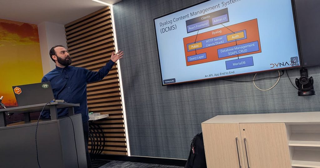
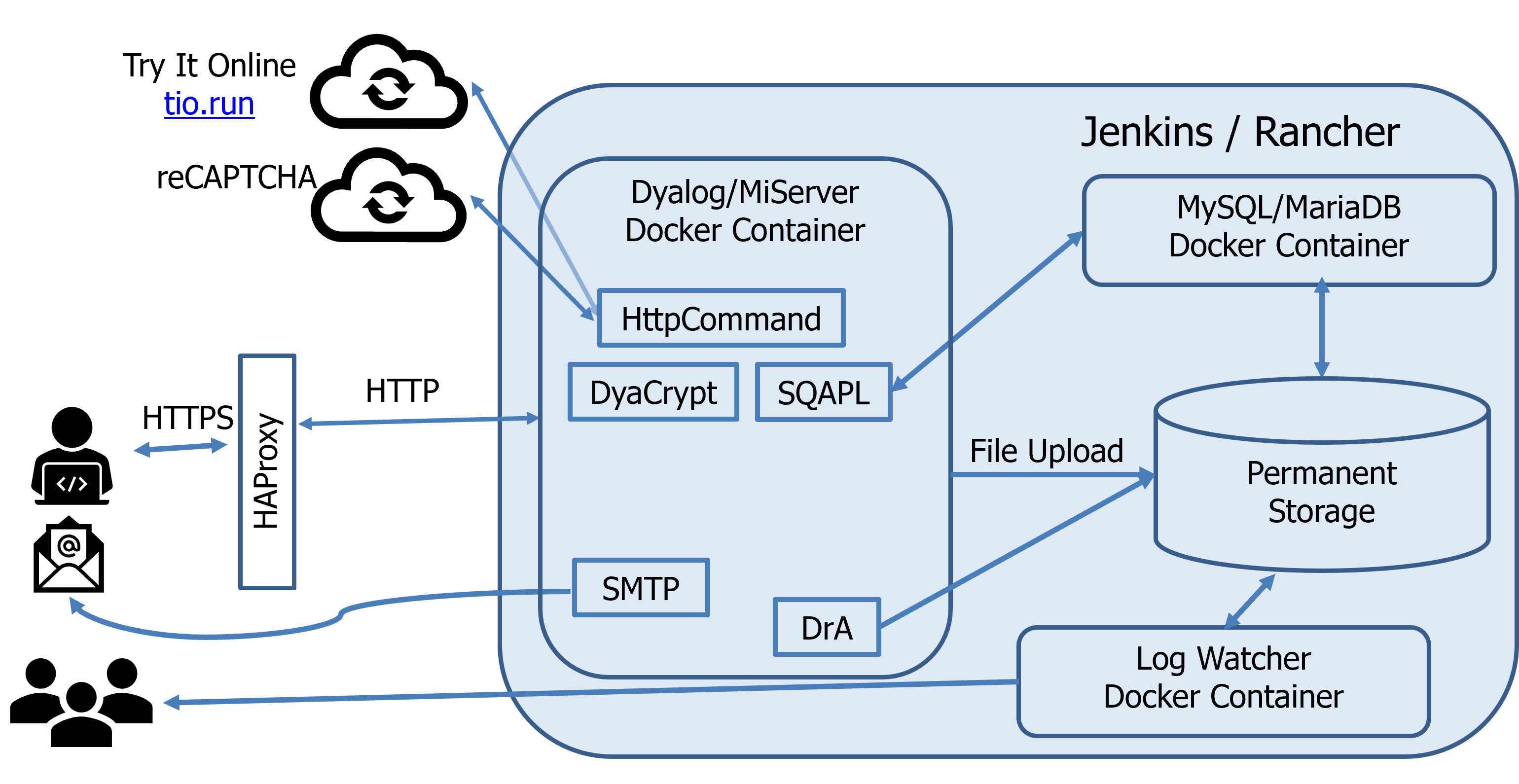
2019-2021 – Back in-house: The contest moved onto Dyalog-grown infrastructure. Almost everything we could write in APL, we wrote in APL:

  • MiServer generated and served the website
  • HttpCommand talked to remote services
  • SMTP sent confirmation emails
  • DCL hashed passwords
  • Conga provided network communications for both MiServer and HttpCommand
  • DrA logged and reported errors to the developers
  • SQAPL communicated with a MariaDB database

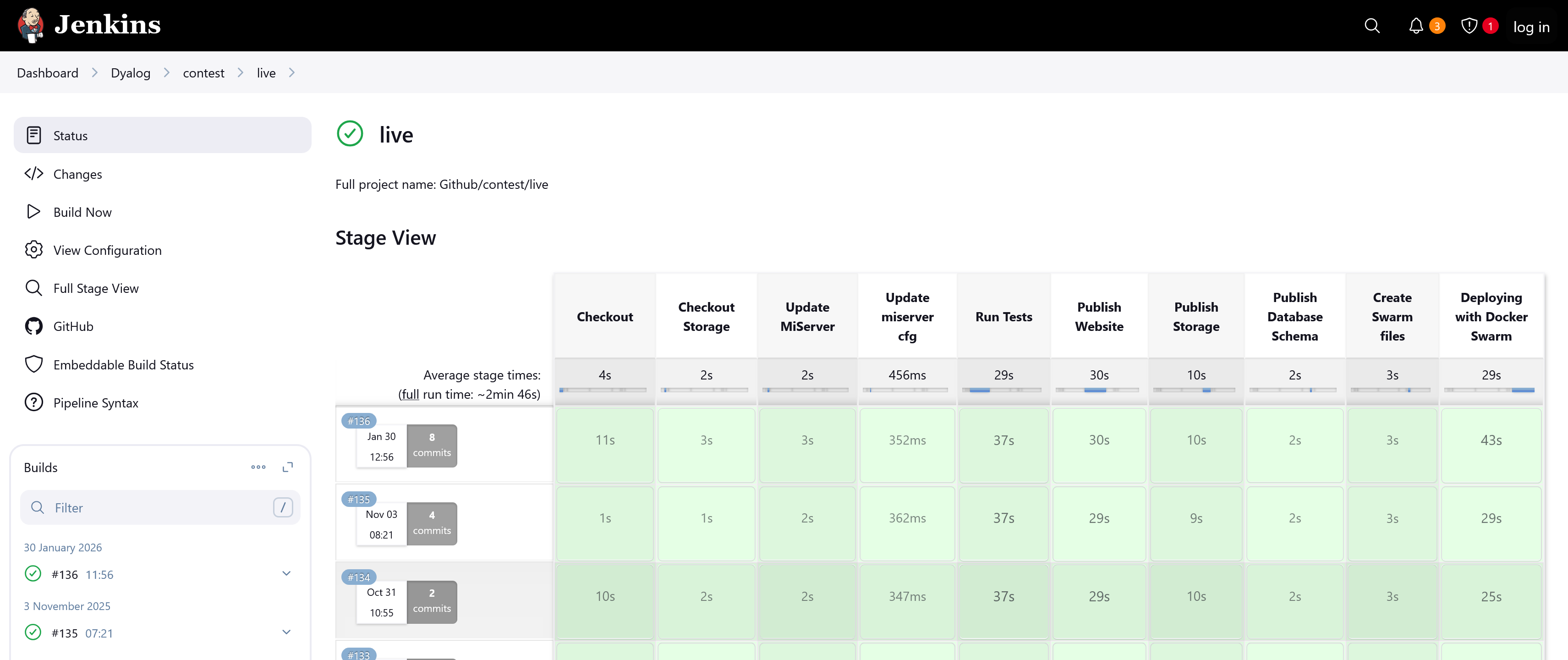
This is what it looked like:

APL Problem Solving Competition screenshot

The sources were managed with Git and stored on GitHub in two repositories: one which held the MiSite code and styling, and one which held the per-round JSON test specifications and per-problem MiPages. The intention was that Jenkins’ continuous integration using Docker containers deployed using Rancher (and later Docker Swarm, when Rancher went all-in on Kubernetes) would make content updates hot-swappable into a running site. In practice, this never worked reliably and content pushes regularly required a service restart anyway, and the split added co-ordination overhead between the two repositories.

We used HAProxy for load balancing and reCAPTCHA to keep the bots out. Phase 1 validation was done by generating test scripts which were then sent to Try It Online for sandboxed execution. Phase 2 was a glorified file upload form. Brian Becker showed a simplified diagram of the moving parts in his Dyalog ’19 presentation:

Brian's diagram

2022-2023 – Enhancements: The Try It Online dependency was replaced with Safe Execute, itself derived from the original TryAPL code, and bespoke checks were added to verify that submitted Phase 2 entries followed the syntactic constraints of each task. Code quality still factored into the final score, so the automated tests were one input among several.

In his introduction to the competition prize-giving ceremony during Dyalog ’23, Brian outlined our thoughts for the future of the competition.

Enter the APL Challenge

In February 2024 we launched the first round of the APL Challenge, replacing the previous Phase 1. After a short break, Phase 2 also got a replacement: The APL Forge. The competition was now:

  • for everyone: While previous competitions exclusively or primarily targetted students, the APL Challenge is equally open to everyone. To facilitate participation by younger, new-to-APL, and foreign-language contestants, its descriptions of APL features and problems are deliberately written in a simplified style.
  • always open: Previously the competition was open for a few months each year. The APL Challenge is open (almost) continuously, with four rounds each lasting three months (with only a day’s down-time between them), and each round is followed by the awarding of prizes.
  • self-contained: Previously, you had to learn APL on your own to be able to participate. With the APL Challenge, each round teaches everything that is needed as part of the problem statements, building up to a more demanding tenth problem (often inspired by – or lifted directly from – the old Phase 1 archive).
  • entirely automated: Every submission is quickly and fully checked, with prizes awarded only based on correctness.

Initially, we recycled the existing server set-up, including the account system and the Phase 1 code for presenting problems and checking submissions. However, that code had already accumulated a significant amount of technical debt, and the changes needed to repurpose it didn’t help. MiServer’s performance characteristics meant that we had to run several parallel containers behind a load balancer, and the automated checker was slow because each submission was juggled across threads. When I showed the APL Challenge to a couple of classes at my children’s school, I also noticed that the account system was a significant barrier: the children either had no email addresses of their own, or couldn’t access them during school hours, which halted the sign-up flow before it began. Although none of this was really broken, it was a consideration for the list of “things to clean up when there’s time”.

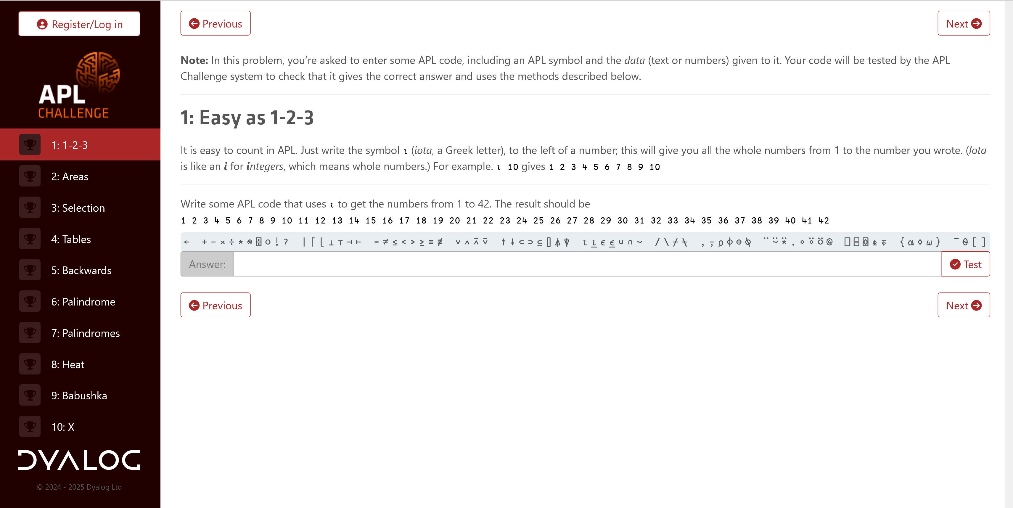
The front end of the site was also redesigned to align more closely with modern styling:

MiServer-based APL Challenge screenshot

In late 2025 I finally found the time we needed. With Dyalog v20.0’s release approaching, I incorporated several of the key features introduced in that release into my rewrite – especially ⎕VGET, the enhancements to ⎕NS, array notation, and the behind operator (), but even the new ⎕SHELL found a use in the code base. Most of the code is fairly straightforward, but one section constructs APL expressions, including single-line dfns, at run time to put the participant’s solution into an appropriate testing context. Traditional debugging tools fell short here, but inline tracing came to the rescue. The result has been live since February 2026.

The new stack

We’d accumulated a lot of experience with Material for MkDocs from the online documentation overhaul for Dyalog v20.0 (compare it to the older v19.0 site it replaced) and from rewriting the APL Quest site, which hosts the old APL Problem Solving Competition Phase 1 problems. Both sites are static MkDocs builds, although the APL Quest does automated checking using an external fork of Attempt This Online, and both have proven straightforward to maintain. Reusing Material for MkDocs as the APL Challenge frontend was the obvious move. Combined with Jarvis for the backend and a small amount of dynamic content, the new stack is:

  • APL code that builds a static site for each round using Material for MkDocs.
  • Jarvis with one small enhancement, serving both the static site and a four-endpoint JSON API.
  • HttpCommand to forward subscription requests to MailerLite.
  • Conga for Jarvis and HttpCommand.
  • Git, GitHub, Docker Swarm, and Jenkins (as before).

By adding Material for MkDocs and Jarvis, we were able to remove MiServer, SMTP, DCL, DrA, SQAPL, HAProxy, Rancher, MySQL/MariaDB, reCAPTCHA, Safe Execute, the load balancer, the multiple container replicas, the dual-repository arrangement, and seven JavaScript libraries used by the MiSite code.

The database was replaced with two TSV (Tab-Separated Values) files in persistent storage. Authorisation, where it exists, is a token that is compared to an environment variable.

After some deliberation, and consulting with our in-house GDPR experts, we also found a way to remove the need to register: the participant’s email is now submitted along with each solution. This let us remove the whole signup-password-confirmation-email procedure, so children at school can use their own (or their parents’) email address without needing access to it immediately, and only receiving an email if they win a prize.

The entire backend is now just over 400 short lines (averaging less than 25 characters) of APL across 16 functions, plus one namespace of 35 English phrases (we plan on adding internationalisation later). For comparison, the previous site used over 2,000 lines of APL and eight files of English phrases and email stubs.

One static site for each round

Each round teaches a different progression of glyphs and concepts. Rather than rendering pages dynamically, we build one Material for MkDocs site for each round. Each round lives in its own uppercase single-letter directory (A through I, with Z reserved for the holding-period site that’s served between rounds). The previous system identified rounds by calendar slots (2024’s round 1 was 20241, and so on). Decoupling round identity from the schedule means that a given round can be re-served later and a round can be designed and tested entirely independently of when it goes live.

A single copy of the shared files and folders – assets, JavaScript, and the legal and front pages – are kept in add/. Before the MkDocs build runs, these are copied into each round’s directory and {{X}} placeholders in markdown files are substituted with the round letter:

 dirs←⊃⊢⍤//1=@1⊢1 0 ⎕NINFO ⎕OPT 1⊢dir,'/?'
 Copy←{
     dest←d,'/',⍺
     ⎕←'COPY -',(2↓∊' & '∘,¨⊆⍵),' → ',∊1 ⎕NPARTS dest,'/'
     dest ⎕NCOPY ⎕OPT'IfExists' 'Replace'⊢(dir,'/add/',⍺,'/')∘,¨⊆⍵
 }
 ls←⊢/¨dirs
 incl←ls∊build
 :For d l :InEach incl∘/¨dirs ls
     ''Copy'mkdocs.yml' 'overrides'
     'docs'Copy'ass' 'js' 'legal.md','index.md'/∘⊂⍨'Z'≠l

     files←(0∊2∘⊃∊⎕D⍨)¨⍤⎕NPARTS⍛/⊃⎕NINFO ⎕OPT 1⊢d,'/docs/*.md'
     :For file :In files
         cont←⊃⎕NGET file 1
         file 1 ⎕NPUT⍨⊂'{{X}}'⎕R l ⎕OPT'Regex' 0⊢cont
     :EndFor

     :If build∩0 1
         {⎕←⍵}¨⊃⊃⎕SHELL ⎕OPT'WorkingDir'd⊢'python -m mkdocs build'
     :EndIf
 :EndFor

A hot-swappable Jarvis

Jarvis serves a static directory using its HTMLInterface setting. However, that setting was defined as a field that was read once when the server starts, and we needed to be able to switch which round’s site/ directory was being served while the server was running, on a fixed UTC schedule. So we amended Jarvis to make HTMLInterface a property: assigning to it now adjusts the private fields that were previously only set at boot time.

That small change is what makes the rest of the design work; round switching is a background thread that watches a single TSV file:

 :Repeat
     :Trap 0
         newChange←13 ⎕NINFO filename
         :If change≢newChange
         :OrIf 0∊40 ⎕ATX'utc' 'dir'
             change←newChange
             (utc dir)←⊃(TSV ⎕OPT'Invert' 2)filename ⍬ 1 1
             inst.Log'Schedule loaded from ',filename
         :EndIf
         begin←1 ⎕DT(2⊃⎕VFI)¨' '@(~∊∘⎕D)¨utc
         interval←begin⍸now
         :If 900⌶0
             newRound←interval⊃dir
         :EndIf
         :If round≢newRound
             round←newRound
             html←⌽round@7⊢'/',(⊃∊'/\'⍨)⍛↓⌽inst.HTMLInterface
             inst.Log'Web interface changed: ',inst.HTMLInterface,' → ',html
             inst.HTMLInterface←html
             file←inst.CodeSource,'/',round,'.json5'
         :EndIf

         newTestFileInfo←FileInfo file
         :If fileInfo≢newTestFileInfo
             fileInfo←newTestFileInfo
             inst.Log'Test data updated from ',file
             data←0 ⎕JSON ⎕OPT'Dialect' 'JSON5'⊃⎕NGET file
         :EndIf

         :If ~900⌶0
             :Leave
         :EndIf
         t←20 ⎕DT'Z'
         ⎕DL 1+1800|¯1-t ⍝ wait until next half-hour
     :Else
         …
     :EndTrap
 :EndRepeat

Every half an hour, the thread re-reads schedule.tsv if its modification time has changed. If the round that should be live differs from the one currently being served, then the HTMLInterface property is updated; the corresponding test data is then (re-)loaded if either the test data file or the round has changed. The schedule itself is a two-column TSV mapping UTC start times to round letters:

utc                 dir
…
2026-01-30 09:00    Z
2026-02-11 09:00    G
2026-04-30 08:00    Z
2026-05-01 08:00    C
2026-07-31 08:00    Z
2026-08-02 08:00    H
…

Editing this file is the entire process for scheduling rounds. There’s no separate content repository, and there’s no longer an aspiration to swap content underneath a running site without telling the site about it. The builds tend to take less than 30 seconds, and the live site is swapped with only a few seconds of downtime:

Jenkins build times for the MkDocs-based APL Challenge

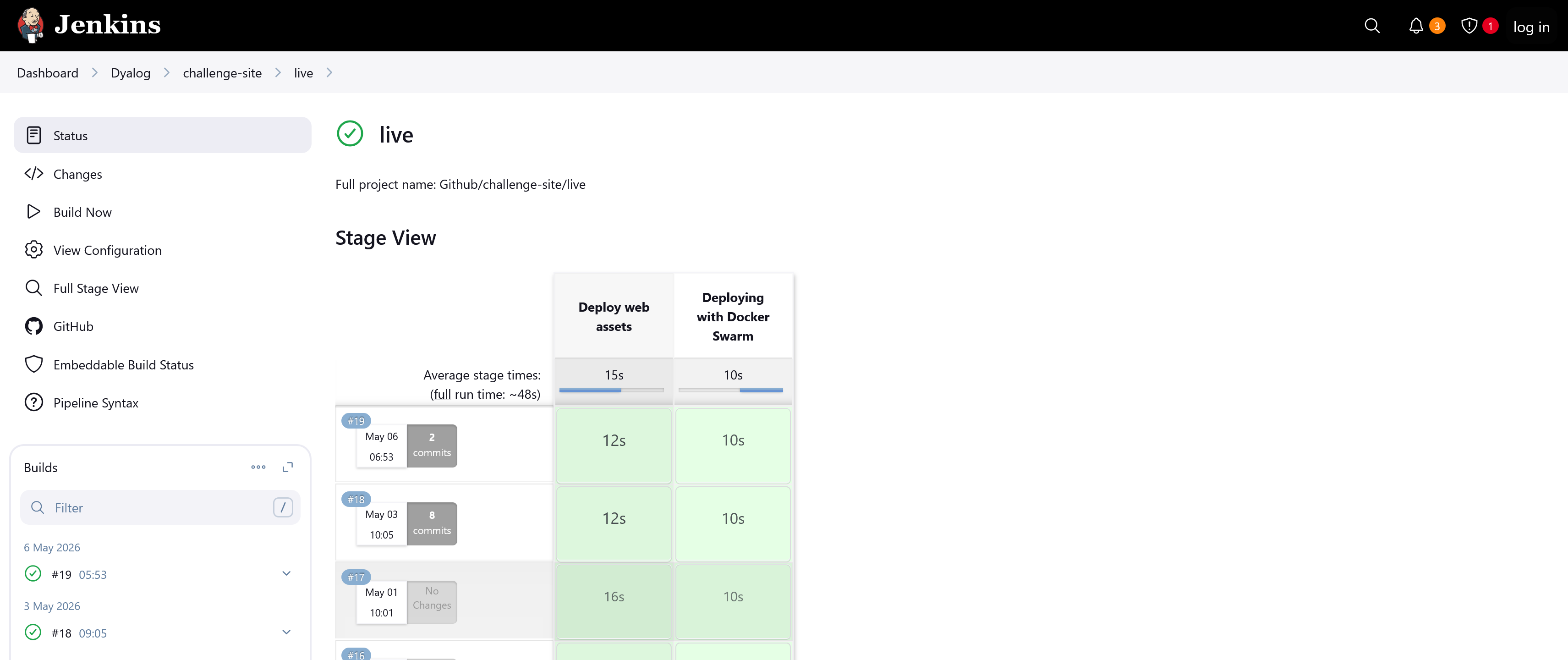
A huge improvement over the previous architecture:

Jenkins build times for the MiServer-based APL Challenge

The JSON5 test catalogue

Each round has a JSON5 file with members P1 through P10 describing how to test each problem. The format was inherited from the MiServer-based system; the test framework that consumes it has been completely rewritten. Here’s part of one:

{
    P1: {
        r:"^ *⍳ *\\d+",
        s:"⍳24",
    },
    …
    P7: {
        a: [
            "'HELLO'",
            "'DYALOG'",
            "'APL'",
            "{⍵[?≢⍵]}¨'AEIOU' 'BCDFGHJKLM' 'NPQRSTVWXYZ' 'AEIOU'",
        ],
        f: "{(2⊃⍵),(2⊃⌽⍵)}",
    },
    …
}

Problems 1–6 ask the participant to type one specific expression that produces one specific value, so the specification carries a reference solution s and a regex r that describes the acceptable solutions. Problems 7-10 ask for a function: the specification carries a reference function f, an array of test arguments a, and (optionally) a preprocessor p to apply before comparing the user’s result with the reference’s. Since the JSON5 strings are APL expressions, we can generate random tests as needed to prevent participants from hard-coding answers.

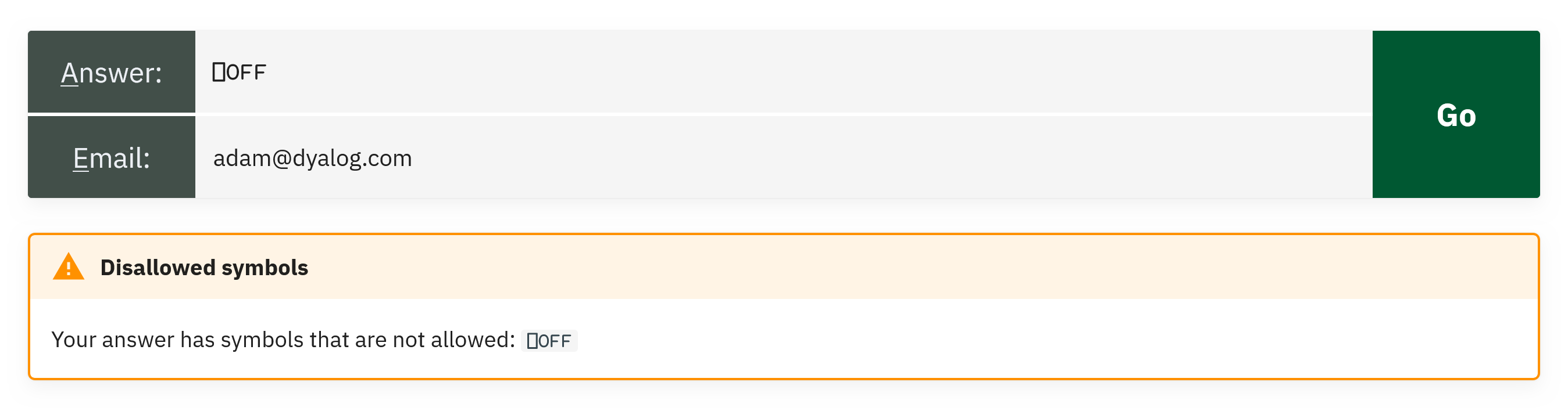
Submitting an answer

JavaScript included in the frontend makes the user’s browser POST [lang, problem, code, email] to the /Submit endpoint. First, we do some sanity checking:

 (rc msg)←req Submit(lang problem code email);anon;T
 lang ⎕C⍨←¯3
 :If ~lang⊂⍛∊##.⎕NL ¯9
     lang←'en'
 :EndIf
 T←lang∘Text
 :If 'Z'≡round
     (rc msg)←8(T'closed')
 :ElseIf ~problem⊂⍤,⍤⍕⍛∊⍕¨⍳10
     (rc msg)←8(T'badProbNo')
 :ElseIf 0∊∊' '=⊃0⍴⊂code
     (rc msg)←8(T'badCode')
 :OrIf 255<≢code←∊code
     (rc msg)←8(T'longCode')
 :ElseIf 0∊∊' '=⊃0⍴⊂email
     email←'^\s+|\s+$'⎕R''∊email
 :OrIf (''≢email)∧⍬≡'\S.*@.*\S'⎕S 3⊢email
 :OrIf email∊⍨⎕UCS 9
 :OrIf 254<≢email
     (rc msg)←¯8(T'badEmail')
 :Else
     …

We then test the submission and add an entry to the sub[mission]s and, if correct, wins database files:

     …
     (rc msg)←'data' 'problem' 'lang'⎕NS⍛Test code
     …
     ((unixtime:20 ⎕DT'Z' ⋄ code:'\t'⎕R'␉'⊢code)⎕NS'problem' 'rc')AppendTSV dbDir,'/subs.tsv'
     :If 0=rc
         req.Server.Log anon,' solved ',round,' problem ',problem
         :Hold 'wins'
             'email' 'problem' 'round'⎕NS⍛AppendTSV dbDir,'/wins.tsv'
         :EndHold
     :EndIf
 :EndIf

Responses consist of a return code and a message, ready for the frontend to render as a Material admonition:

Example admonition

The submission record uses two new Dyalog v20.0 features:

(unixtime:20 ⎕DT'Z' ⋄ code:'\t'⎕R'␉'⊢code)⎕NS'problem' 'rc'

The parenthesised expression is a namespace literal containing unixtime and code with their value expressions, and ⎕NS'problem' 'rc' amends the reference left argument (new!) with copies of those two variables. The result is a four-member namespace, ready to be appended as a TSV row. I chose to pass the row as a namespace rather than an ordered vector so that the table column order wouldn’t matter.

The test harness

Test is the largest function in the codebase (110 lines), but mostly consists of validation; the actual evaluation is short. The function begins with more usage of new Dyalog v20.0 features:

 (rc msg)←params Test code;…
 ⎕THIS ⎕NS params
 :Trap ⎕VGET⊂'debug' 0
     T←lang∘Text
     spec←data ⎕VGET⊂'P',problem
     …

⎕THIS ⎕NS params merges the entire params namespace into the current function’s scope, so data, problem, and lang (set up by the caller in Submit) are now ordinary local names with no params. qualifier required. data ⎕VGET⊂'debug' 0 decides whether to trap unexpected errors at the top level (during development, I set debug←1 from the session), and ⎕VGET then reads the specification for the requested problem out of the test data.

When initial validation is complete, the function proceeds based on the type of specification that was supplied (a regex-and-value check for problems 1-6, or a test-cases-and-function check for 7-10) and (after more specific validation) either runs the user’s code with ()⍎ (to run it in a separate namespace) or composes a small expression that wraps the user’s function and the reference function side-by-side and runs both in turn. (Debugging the generated expression is where inline tracing came in handy for me.) If the answers match, the frontend gets 0 'Your answer is correct. Good job!'. Otherwise the message tells them whether the answer was wrong, the methods used were wrong, the symbols used were wrong, or the code crashed.

Security is delivered by a safe character set, which stops glyphs that are dangerous (, , , ) or can lead to runaway execution (, , ):

safe←'+-×÷⌈⌊*⍟|!○~∨∧⍱⍲<≤=≥>≠.@≡≢⍴,⍪⍳↑↓?⍒⍋⍉⌽⊖∊⊥⊤⌹⊂⊃∪∩⍷⌷∘/⌿\⍀¨⍨⊆⍥⊣⊢⍤⌸⌺⍸()[];⋄:⍛⍬{}⍺⍵¯ '

This, together with limited memory, makes the new system light-weight enough that we can run it in the main thread, thus saving on thread juggling.

Authorisation as a one-liner

There are only two protected endpoints – Table for reading the TSVs, and Purge for deleting records – both for our own administrative use. (Participants don’t authenticate at all; an email goes in with each submission, the browser remembers it client-side, and that’s it. The worst that can happen is that I submit a correct answer with your email address, and that you then get a single notification email about having won a competition you haven’t heard of. Your email is then purged from our systems.) A single dfn, evaluated once for each protected request, is sufficient:

Authorised←{(⊂⍵.GetHeader'AuthToken')∊(⎕VGET⊂'authToken' '' ⋄ Env'AUTHTOKEN')~⊂''}

The valid token is whichever of the variable authToken (set manually for local testing) and the environment variable $AUTHTOKEN (set by Docker from a Jenkins credential) is non-empty. ⎕VGET returns its default of '' if authToken isn’t defined. The request’s AuthToken header is compared against the resulting list.

The “database”

The two storage tables are TSV files. They’re created at server start if they don’t exist. The combination of :For:In with multi-line array notation makes it easy to spot what goes where, whilst preventing the lines from getting too long:

 :For name head :In (
         'subs'('code' 'rc' 'problem' 'unixtime')
         'wins'('email' 'problem' 'round')
     )
     pathfile←dbDir,'/',name,'.tsv'
     :If ~⎕NEXISTS pathfile
         pathfile ⎕NPUT⍨[head ⋄ ]TSV''
     :EndIf
 :EndFor

[head ⋄ ] is array notation for a one-row matrix containing the row head – a header row. TSV is ⎕CSV with the separator pre-set to the Tab character and quotes disabled (Submit already protected us against Tab characters in the submission by replacing them with the Unicode control picture ):

 TSV←⎕CSV ⎕OPT('Separator'(⎕UCS 9) ⋄ 'QuoteChar' '')

subs.tsv contains code, rc, problem, and unixtime – every submission, with no email column. wins.tsv contains email, problem, and round – correct submissions only, with no code column and no timestamp. The two tables share no column that would let you join a participant’s email to the code they typed. We can produce statistics (“how many people solved problem 7 of round G?”), and we can email prize winners, but we can’t, even ourselves, look at a piece of submitted code and say which person wrote it. That’s deliberate.

Appending a record is a one-liner that takes a namespace whose names match the table’s columns, slots the values into a fresh row in the right column order, and asks ⎕NPUT to append (2):

 r←file 2 ⎕NPUT⍨[ns.⎕VGET⊃⌽(TSV ⎕OPT'Records' 1)file ⍬ 4 1 ⋄ ]TSV''

(TSV ⎕OPT'Records' 1)file ⍬ 4 1 reads only the header row (one record), and ns.⎕VGET then plucks the values out of the namespace in that order.

Reading a whole table for the administrative Table endpoint is:

 resp←0 ⎕JSON 1 ⎕JSON⊂2(TSV path ⍬ 4)

Here, we read the file then round-trip through ⎕JSON to leverage a dataset wrapper – introduced in Dyalog v19.0 – that transforms a table into a vector of namespaces. To see what’s happening, here is a sample wins table:

      wins←[
            'email'           'problem' 'round'
            'foo@example.com' 1         'A'
            'bar@example.com' 2         'B'
           ]
      1 ⎕JSON⊂2 wins
[{"email":"foo@example.com","problem":1,"round":"A"},{"email":"bar@example.com","problem":2,"round":"B"}]

Jarvis will respond with JSON data, but does the conversion from APL array for us, so we preempt the double-conversion with 0 ⎕JSON. Yes, it is unnecessary work, but it happens rarely enough not to matter, and even with the round-trip it is faster than the alternative, more-involved, ⊃{()⎕VSET(↑⍵)⍺}⍤1/TSV path ⍬ 4 1.

Behind the scenes with

Dyalog v20.0 introduced the new behind operator, . This uses the left operand to provide a left argument to the right operand:

  • X f⍛g Y is (f X) g Y
  • f⍛g Y is (f Y) g Y

This is a very common pattern, and across the 400-line backend appears over 30 times. Here are some of the representative uses:

New 'data' 'problem' 'lang'⎕NS⍛Test code Make Test take a list of names representing a namespace,
rather than taking a namespace reference
Old (⎕NS'data' 'problem' 'lang')Test code
New lang⊂⍛∊##.⎕NL ¯9 Make look for a single whole text,
rather than for each letter
Old (⊂lang)∊##.⎕NL ¯9
New mask~⍛/what / means “filter in”; “keep the indicated”
~⍛/ means “filter out”; “remove the indicated”
Old (~mask)/what
New (∨/spec.s∘∊)⍛/¨groups ⍛/ is a monadic filtering operator
f⍛/¨Y filters each element of Y by the predicate function f
Old ((∨/spec.s∘∊)¨groups)/¨groups

I especially like how allows me to extend the primitive vocabulary of APL by providing oft-needed variants of existing primitives; X⊂⍛∊Y and X~⍛/Y and f⍛/Y could easily have been primitives in their own right.

Internationalisation

Responses to submissions, including both success and failure messages, as well as reports about internal errors in the system (luckily, we’ve only had one minor error, and it was due to a mistake in the frontend), are sent as plain human-readable text together with a return code. The frontend renders it as a Material-style admonition with the colour and icon determined by the return code. English phrasings live in an array notation namespace in the file en.apla:

(
 and:'and'
 ansCorrect:'Your answer is correct. Good job!'
 ansErr:'Error<p>Your answer caused a'
 ansPass:'Your answer passed all tests. Good job!'
 arg:'argument'
 as:'as'
 badEmail:'Invalid email address'
 …
)

Jarvis loads .apla files together with the other application code. Now, you might have spotted the line :If ~lang⊂⍛∊##.⎕NL ¯9 and thought that this looks error-prone; surely, a malicious actor could issue a POST with the language set to the name of an unrelated namespace! Worry not; the line lang ⎕C⍨←¯3 makes sure only namespaces with entirely lowercase names are reachable as language packs, while all the system’s top-level namespaces begin with a capital letter. Phew, close!

Adding a new language to the backend consists of adding one file. Of course, the problem statements and informational pages will also need translation, but Material for MkDocs supports internationalisation by having a separate directory per language. I only recently finished composing all nine planned rounds of content, and want to harmonise them a bit more before we begin translating, but at least the wiring is there.

Looking back and forwards

The previous stack was a very useful test of the code and tools that we supply: it exercised our libraries, gave us bug reports against our own tools, and kept us using what we were selling. However, it also accumulated technical debt, and as the system evolved, the seams started to show.

The new stack also uses Dyalog technology (Jarvis, HttpCommand, Conga, and most of the newest language features) and these are really the things we’re selling today. It does so much more economically too: the whole thing runs on a single virtual CPU with 512 MB of RAM, whereas the old system used at least two virtual CPUs (more during peaks) with 1 GB of RAM each.

Have a look at Jarvis! It is really easy to get started. Here’s the bare minimum to get from a clear workspace to a running service with a good architecture in a folder /rot (replace with any other folder you want to use instead):

  1. Design your API: We’ll make it really simple; create a single function Rotate←{⊃⌽/⍵} in the workspace.
  2. Create the folder and function source file: ]Create # /rot
  3. Create the Jarvis configuration file: The easiest is ]Repr (CodeLocation:'.' ⋄ HTMLInterface:'.' ⋄ IncludeFns:'Rotate') -f=json -o=/rot/jarvis.json
  4. Create the HTML interface: Here’s one with two input fields, a button, and the minimal JavaScript needed to make the button work:
    <!DOCTYPE html>
    <html>
      <head>
        <title>Jarvis Text Rotator</title>
        <script>
          Exec=()=>{
            fetch("/Rotate",{
              method:"POST",
              headers:{"content-type":"application/json; charset=utf-8"},
              body:JSON.stringify([steps.valueAsNumber, text.value])
            }).then(r=>r.json()).then(d=>out.innerHTML=d)
          }
        </script>
      </head>
      <body>
        <input id=steps placeholder=Steps type=number>
        <button onclick=Exec()>⌽</button>
        <input id=text placeholder=Text>
        <br>
        <output id=out></output>
      </body>
    </html>

    Save this text to /rot/index.html.

  5. Get Jarvis: ]Get github.com/Dyalog/Jarvis/blob/master/Source/Jarvis.dyalog
  6. Start the server: Jarvis.Run'/rot/jarvis.json'
  7. Try it: Open localhost:8080 in your browser, fill in the fields, and click the button!

Try HttpCommand, too! While the above server is running, we can easily use it as a micro-service, bypassing the HTML frontend:

  1. Get HttpCommand: ]Get HttpCommand
  2. Issue the command: resp←HttpCommand.GetJSON'POST' 'localhost:8080/Rotate' (2 'Hello')
  3. Inspect the response: resp.Data – this will give the character vector 'lloHe'

If you’ve made it all the way to here, congratulations! Don’t forget to promote the APL Challenge and the APL Forge – they are available year-round!

DYNA26: A Review

In April we hosted DYNA26, our latest Dyalog North America user meeting. We returned to midtown Manhattan for a day of presentations, demonstrations, and the sort of impromptu conversations that only happen when APLers are in the same room.

Part of the Dyalog Ltd contingent (Brian Becker, Rich Park, Asher Harvey-Smith, and Holden Hoover) spent a few days beforehand in Rochester, New York, having a pre-DYNA “conclave” at Brian’s house, working through tooling design discussions and event preparation. We’re a geographically-distributed team, so we make the most of the opportunities to work together in person; our thanks to Brian for hosting once again.

Attendees watch Morten's presentation

The room filled with a familiar mix: enthusiasts, current developers building on Dyalog at customer sites, users of other APL implementations, and a few who hadn’t written any APL but were curious enough to spend a day with us. As ever, that mix is what makes DYNA enjoyable to host.

Presentations

The Dyalog Road Map
Morten Kromberg (remote)

Morten joined us remotely to open the day with the road map. The headline theme was LLMs. Stephen Taylor’s line that “Claude is the new Quad” captured it nicely, suggesting how the often-tedious system-interaction layer of programming, usually handled by I-beams and quad-functions and increasingly by libraries, can now be handled by LLMs as well, leaving APLers freer to focus on the core problem-solving to which the notation is so well-suited.

Morten covered recent experiments and experience: writing prototypes, tests and documentation; generating ⎕WC GUI code; and producing interactive tutorials for existing tools. There appear to be some productivity gains, particularly when an experienced developer is supervising. LLMs are already strong at non-APL tooling code (C#, HTML/CSS/JavaScript) that APLers regularly need to write around their core applications, and they’re steadily improving with APL code.

Of course, generative tooling is not the only thing on the road map. Morten talked about an increased focus on organisational and software security through the BSIMM initiative, including static analysis of both the interpreter’s C code and APL code. This can be used to, for example, find injection vulnerabilities through uses of (execute), ⎕SHELL, or SQAPL. He also covered recent language additions, including APL array notation and ⎕VGET/⎕VSET, and looked ahead to future work including a potential ⎕IMPORT module system — a prerequisite for the robust project and package management that the community has been asking for.

An APL App End to End
Rich Park

Rich followed with a showcase of Dyalog’s tools wrapped around a single example application: a video data CRUD/REST service with search and recommendation. The demonstration included the upcoming Stark REST router and its OpenAPI specification generator, the extensions to ⎕DT coming in Dyalog v21.0, and the use of isolates to push heavy computation into a separate Dyalog process so that Jarvis/Stark can keep servicing HTTP requests in the main thread. He showed APL code to compute search results and recommendations using simplified expressions of term-frequency inverse-document-frequency and cosine-similarity, to convey how using Dyalog to deal with the fiddly interfaces and inconveniences of real applications lets us focus on using APL to express core algorithms. Plenty to consider for anyone building services in APL.

Rich pointing to slide of application architecture overview diagram

Migration Tools for APL Systems
Morten Kromberg (remote)

Morten returned for a second presentation, this one looking at tooling for migrating to Dyalog from other APL implementations. There are tools to swap language constructs for Dyalog cover functions that reproduce the original behaviour — and you wouldn’t necessarily expect it, but even ∧/ (and-reduction) and ∨/ (or-reduction) can need special handling to behave identically for certain arguments.

GUIs are often the trickiest part of any migration. Often, the pragmatic answer is to move to a conventional web stack, such as React, but sometimes a customer would rather retain the native Windows GUI behaviour intact through the migration. For that, there’s the ∆WI emulator for APL+Win’s ⎕WI that is being developed by Davin Church. In the past we’ve even seen an APL2 GDDM terminal interface migrated to an HTML/SVG-based emulator. Looking further ahead, the path from ∆WI to eWC could let migrated (or original Dyalog-native) GUIs run cross-platform inside HTMLRenderer or a browser without much further refactoring.

Parsing User Input for Database Normalisation
Mark Wolfson and Kori Smith, BIG

Mark is a familiar face at Dyalog events; this time he was joined by Kori Smith to talk about the work BIG does in inventory analysis and data aggregation for the jewellery industry — highly customised data processing for approximately 1,000 customers. The case study they explored was the perennial problem of inconsistent, hand-entered, product descriptions that need to be mapped onto a regular set of fields for database storage and later analysis.

BIG’s approach combines APL with regular expressions to iteratively refine the processing in a way that can be tuned on an individual customer basis. As Mark and Kori explained, the use case demands more consistency than an LLM can comfortably guarantee, and the mainstream NLP toolkit is overkill for what’s actually a fairly bounded problem albeit with some ambiguities (“emerald”, for example, is both a gemstone and a cut of diamond).

Kori Smith presenting

Dyalog OpenAPI Client Generator
Holden Hoover

Holden presented the Dyalog OpenAPI Client Generator, a tool that promises to make it considerably more straightforward to interoperate with the many existing services that publish OpenAPI specifications. Several attendees indicated that they had encountered precisely this issue already, and would benefit from not having to hand-write clients for sprawling third-party APIs.

One nice side effect of a machine- and human-readable specification is that it encourages thinking through API design before implementation. Holden demonstrated the generator against the Open-Meteo weather API, and against the OpenAI API — the latter to generate an introduction-to-APL page complete with examples and an image. He also mentioned the Stark REST Router layer that sits on top of Jarvis, making it easier to expose a Dyalog application to the wider world of HTTP clients.

APL Primitives in the 21st Century
Enhancements in Dyalog v20.0: Arrays, Namespaces, Composition, and Inline Tracing

Asher Harvey-Smith

After lunch, Asher gave us a double-bill of presentations about the past and current development of language features in Dyalog.

First, he took us on a whirlwind tour of how the APL primitives have evolved through Dyalog v13.0 to v18.0, with a particular focus on extensions and new primitives motivated by leading axis theory. This is the idea that functions applied along the first axis can be used to apply to sub-arrays, or between collections of sub-arrays of two argument arrays, in a consistent and malleable way compared to the ad-hoc nature of bracket axis. He started with short left arguments to take () and drop () in Dyalog v13.0, and progressed through to unique mask () which marks unique major cells along the leading axis from the outset.

From there, Asher moved on to new features in Dyalog version 20.0. We saw APL array notation and its integration into the Dyalog session and editor, the ability to write namespace literals analogous to JSON, and inline tracing to step through an expression one function at a time. He explained behind () as a complement to compose (), with the filter idiom ⍛/ as his favourite example (for example, >∘0⍛/ to extract positive elements from a list). He concluded with ⎕VGET/⎕VSET for manipulating variable values without resorting to the potentially-dangerous execute (), and ⎕SHELL for more complete and controllable command-line execution from APL.

Asher presents a slide about short left arguments

Jarvis and AI
Brian Becker

Brian presented an experiment exploring how far a modern LLM could go in building a simple – but fully functional – Jarvis‑based web service. The target application was a Wordle™‑style game, and the model chosen was Google’s Gemini, selected for its easy, low‑cost browser access.

Brian began by crafting a prompt that described his requirements for the service. He then asked Gemini to refine the prompt and produce a project plan. Gemini responded with a surprisingly thorough plan, addressing several architectural details that Brian had not explicitly mentioned. When instructed to “do it all,” Gemini generated an HTML file containing the complete HTML/CSS/JavaScript front end, an .apln file defining the WordleServer namespace, and an .apls DyalogScript file to configure and launch the service. Then followed an iterative debugging loop (run the service, hit an error, paste the error into Gemini, apply the suggested fix, and repeat). Eventually Gemini produced a workable, if not elegant, solution. Brian proposed a cleaner approach, which Gemini incorporated. That single suggestion ended up being Brian’s only code contribution; all other APL, HTML, CSS, and JavaScript was generated entirely by Gemini. The final product was a clean, responsive game that Gemini named ARRAYDLE. Brian noted that the process might have been even smoother if Gemini had the ability to execute APL code directly.

This experiment reinforced two trends: LLMs are rapidly improving at generating APL code, and they already excel at producing polished HTML‑based front ends.

AVG — A Voxel Game
Kyle Croarkin

Kyle gave us a glimpse of his experience learning APL since he started in August 2025, and the substantial project he built to test his learning – AVG, A Voxel Game (essentially, a mini-Minecraft!). He’d wanted to develop something more meaningful than puzzles but nothing too daunting, so that he could really explore APL’s expressivity and the interpreter’s performance against the demands of a real-time game.

It was particularly nice to hear Kyle describe moments that more seasoned APLers will recognise. Kyle described arriving at a solution for finding invisible cube faces, only to realise it mirrored the structure of John Scholes’ Game of Life, giving him the revelatory experience of suggestivity. He talked about how quickly one can iterate on ideas when the notation is terse enough to keep everything on screen, and how APL puts the data right in your face. He was honest about the learning cliff, especially coming from a conventional CS background, and about the things that weren’t well-suited for APL in any obvious way (flood-filling algorithms for light and shadow being a notable example).

Kyle presents A Voxel Game

The APL Trust
Mark Wolfson

Mark closed the day with a talk about The APL Trust, a charitable organisation looking for applications for projects that either do work with/in APL or that benefit the APL community and ecosystem more broadly. As an example, a recent grant has supported the development of the APL387 font. Mark is also now an official Dyalog agent for North America, helping to support existing and prospective customers with their use of Dyalog.

Q&A and Conversation

The day was concluded with a Q&A session that gradually broadened into a more general discussion, touching on the ongoing challenges of promoting APL such as the glyphs, onboarding more generally, engaging with communities beyond the existing APL world, and the difficulty commercial users sometimes face in sharing their use cases without revealing industry secrets. None of these are new problems, but it’s always useful to discuss them together.

In Conclusion…

DYNA26 was a great day, well attended and warmly received. Conversations extended beyond the scheduled breaks and continued afterwards when we went for dinner and drinks.

The next user meeting will be Dyalog ’26 in Eastbourne, U.K., on 12-16 October. We hope to see many of you there.


Materials and recordings from DYNA26 will be added to the event webpage as they become available.

D’Hondt Apportionment Made Easy with APL

Today, the UK is holding elections for local councillors in England, and members of the devolved parliaments in Scotland and Wales. Until a political party starts pushing for mandatory APL lessons, we’re not interested in the results of these elections for this blog post. What we are interested in is algorithms, and, for the first time, the elections to the Welsh Parliament (usually referred to as the Welsh ‘Senedd’) used the D’Hondt method for allocating seats.

The D’Hondt method is named after Belgian mathematician and lawyer Victor D’Hondt, although it was independently invented by United States Founding Father Thomas Jefferson almost a century earlier! The method transforms a vote count for a number of political parties into an approximately proportional allocation of seats to each of the parties. Therefore, unlike in previous Senedd elections, Welsh voters do not have individual representatives on their ballots. Instead, they each vote for one political party. The parties then send as many representatives to the Senedd as they are allocated by the D’Hondt method.

With the D’Hondt method, seats are allocated to parties one-by-one. When each seat is allocated, it is given to the party with the largest vote count relative to the number of seats they have already been given. This way, more popular parties are given seats first, but when they have several already, a seat goes to a smaller party so that it is also represented.

This means that, when allocating a seat, the ‘quotient’ votes÷(seats+1) is calculated for each party, where votes is the number of votes the party received, and seats is the number of seats they have been allocated so far. The +1 is included to avoid division by zero. The party with the largest quotient is allocated the seat, and the process is repeated until all seats have been allocated.

Let’s implement this in APL. Given a vector votes and a vector seats, with each index corresponding to a political party, the index of the party with the greatest quotient can be found as follows:

      i←⊃⍒votes÷seats+1

The grade down of the quotient returns the indices to sort the quotients in descending order. Therefore, the first of these indices will be the index of the greatest quotient – exactly what the algorithm calls for.

We then need to update seats to give a seat to this lucky party. There’s more than one way to do this, but I’ll take a functional approach and use the at operator (@) to add 1 ‘at’ the index of party i:

      1(+@i)seats

This can be wrapped in a dfn, in which is the votes vector and is the current seat allocation.

      Step←{
          i←⊃⍒⍺÷⍵+1
          1(+@i)⍵
      }

To allocate, say, fifty seats, the Step function should be applied 50 times on successive seat allocations – an ideal use-case for the power operator (). Let’s try it with a hypothetical vote share of 4:3:2 for three parties:

      4000 3000 2000 (Step⍣50) 0 0 0
22 17 11

That’s a ratio of around 4:3.1:2 – a good approximation of the original vote-share!

It’s easier to visualise the behaviour of the D’Hondt method over time by considering just two parties. Let’s call them Party A and Party B. Suppose that these parties received 12,345 and 6,789 votes respectively, and share a 50 seat parliament.

      12345 6789 (Step⍣50) 0 0
32 18

Party A is allocated 32 seats, while party B is allocated 18. This ratio is, again, reasonably close to that of the votes:

      12345÷6789  ⍝ vote ratio
1.818382678
      32÷18       ⍝ seat ratio
1.777777778

Let’s see how this ratio changes with each step. By modifying the Step function, we can record the intermediate seat allocations. is now a matrix with a row for the seat allocation after each step. The most recent allocation is extracted with ⊢⌿, which is an idiom for the last row of a matrix. The function must now be called with an initial value of [0 0⋄], which is a one-row matrix of two zeros expressed using array notation.

      Step←{
          seats←⊢⌿⍵
          i←⊃⍒⍺÷seats+1
          ⍵⍪1(+@i)seats
      }
      12345 6789 (Step⍣50) [0 0⋄]
 0  0
 1  0
 1  1
 2  1
 3  1
 3  2
 4  2
 5  2
...

We can now plot the ratio (the ÷/ of this result matrix, on the vertical axis) against the step of the method (on the horizontal axis). The ratio after each step is drawn as an orange dot, and the perfect ratio which the method is approaching is drawn by the lavender line.

We can see the ratio converging to the ratio of the votes. The really interesting question is why. I won’t give a formal proof here, that’s one for mathematicians and political scientists to write about. I will, however, show you how I understand it.

It’s interesting to look at a plot of the seat allocation given by the D’Hondt method alongside a ‘perfect’ allocation where we are allowed fractional seats. The vertical axis corresponds to seats allocated to party A, and the horizontal axis corresponds to seats allocated to party B. The trace of seat allocations is drawn as an orange line in the shape of a staircase, and the line of perfect allocation is drawn as a straight lavender line.

At each step, the D’Hondt method (usually) moves towards, and subsequently crosses, the line of perfect allocation. When an allocation is above the line, Party A has ‘too many’ seats, giving it a smaller quotient. The method then allocates a seat to Party B to correct for this, corresponding to the rightward move on the plot. The opposite also applies – when the allocation is below the line, Party B has the smaller quotient, and the method moves the allocation vertically.

There are exceptions to this pattern – cases where the allocation moves away from the line of perfect allocation. This is because of the “fudge factor” +1 on the seat count. This imaginary extra seat for each party can skew the allocation decision occasionally. From my limited reading, it looks like this is a known behaviour of the D’Hondt method, and is deliberately retained.

By ‘hugging’ the perfect allocation like this, the D’Hondt method stays within a few seats of being perfectly proportional. As the number of seats increases, this error is relatively smaller, so the accuracy of the method increases.

This is how the D’Hondt method allocates seats at a ratio close to the ratio of votes, and gets better as there are more seats available.

Irrespective of whether you’re Welsh, I hope it was interesting to explore the D’Hondt method for apportionment with APL!

Outperforming Nested Arrays with Classic APL Techniques – Part 2

In my previous blog post on flat techniques, I demonstrated how you can use a flat representation for nested data, explored searching and structural manipulation of this kind of format, but did not perform any numerical calculations – that’s what I’m going to look at now. This is also the topic of a classic Quote Quad paper by ‘Boolean’ Bob Smith. If you’re interested in discovering more once you’ve finished reading this blog post, I urge you to read that paper.

With numeric data, it’s much harder to use an embedded delimiter for partitioning, as there’s unlikely to be a choice of delimiter that will never be part of our data. Therefore, I’ll use a separate Boolean vector indicating the start of each partition (I showed a format like this in the last post, but didn’t put it into practice). Here’s an example:

      test  ←3 1 4 1 5 9 2 7
      starts←1 0 0 1 0 1 0 1
      starts⊂test  ⍝ the nested vector this represents
┌─────┬───┬───┬─┐
│3 1 4│1 5│9 2│7│
└─────┴───┴───┴─┘

Partitioned Sum

Let’s look at the basic plus reduction, +/. I want to use our partition vector to do the equivalent of +/¨ on the partitions.

      +/¨starts⊂test  ⍝ the goal
8 6 11 7

The trick do this with the partition vector is to use a +\ and sample the results at the ends of sub-vectors:

      [
          test
          +\test
          starts    ⍝ start of each sub-vector
          1⌽starts  ⍝ end of each sub-vector
      ]
3 1 4 1  5  9  2  7
3 4 8 9 14 23 25 32
1 0 0 1  0  1  0  1
0 0 1 0  1  0  1  1
      (1⌽starts)/+\test  ⍝ sample +\test at the end of each sub-vector
8 14 25 32

The important thing to notice here is that 8 is the sum of the first sub-vector, 14 is the sum of the first and second sub-vectors, 25 is the sum of the first, second, and third sub-vectors, and so on. This is the same as +\+/¨starts⊂test:

      +\+/¨starts⊂test
8 14 25 32

To recover the sum of each sub-vector, I can undo the +\ by finding the pairwise differences between the results:

      ¯2-/0,(1⌽starts)/+\test
8 6 11 7

It’s time to try it on some larger data! I’ll need some random numbers, and some random partition points.

      numbers←?1E6⍴1000         ⍝ random (whole) numbers
      starts←0.8<?1E6⍴0         ⍝ random partition points
      (⊃starts)←1               ⍝ must start with a 1
      nested←starts⊂numbers     ⍝ to compare against
      [10↑numbers ⋄ 10↑starts]  ⍝ let's look at it
123 898 773 377 564 395 306 673 84 62
  1   0   0   1   0   0   0   0  0  0

Now, do I see a speed improvement by using the flat version of +/¨?

      ]RunTime -c "+/¨nested" "¯2-/0,(1⌽starts)/+\numbers" 
                                                                                     
  +/¨nested                  → 2.7E¯3 |   0% ⎕⎕⎕⎕⎕⎕⎕⎕⎕⎕⎕⎕⎕⎕⎕⎕⎕⎕⎕⎕⎕⎕⎕⎕⎕⎕⎕⎕⎕⎕⎕⎕⎕⎕⎕⎕⎕⎕⎕⎕
  ¯2-/0,(1⌽starts)/+\numbers → 1.3E¯3 | -53% ⎕⎕⎕⎕⎕⎕⎕⎕⎕⎕⎕⎕⎕⎕⎕⎕⎕⎕⎕

Great, it’s around twice as fast. I didn’t include the cost of converting between formats here – including the starts⊂numbers in this comparison would tip the scales even further.

It doesn’t end here, though. I generated partitions with the expression 0.8<1E6⍴0, which includes a 1 approximately every 5 places. By changing that 0.8 constant, I can change the density of 1s in our partition vector, thereby controlling the size and count of sub-vectors that the data is chopped up into. When I increase it, there will be fewer, larger, sub-vectors; when I decrease it, there will be more, smaller, ones. Changing this constant has an effect on the relative performance of the flat method.

Using 0.5:

      ⍝ .. remake data ..                                   
      ]RunTime -c "+/¨nested" "¯2-/0,(1⌽starts)/+\numbers"            
                                                                                     
  +/¨nested                  → 6.3E¯3 |   0% ⎕⎕⎕⎕⎕⎕⎕⎕⎕⎕⎕⎕⎕⎕⎕⎕⎕⎕⎕⎕⎕⎕⎕⎕⎕⎕⎕⎕⎕⎕⎕⎕⎕⎕⎕⎕⎕⎕⎕⎕ 
  ¯2-/0,(1⌽starts)/+\numbers → 1.8E¯3 | -72% ⎕⎕⎕⎕⎕⎕⎕⎕⎕⎕⎕

Using 0.9:

      ⍝ .. remake data ..                                     
      ]RunTime -c "+/¨nested" "¯2-/0,(1⌽starts)/+\numbers"             
                                                                                     
  +/¨nested                  → 1.7E¯3 |   0% ⎕⎕⎕⎕⎕⎕⎕⎕⎕⎕⎕⎕⎕⎕⎕⎕⎕⎕⎕⎕⎕⎕⎕⎕⎕⎕⎕⎕⎕⎕⎕⎕⎕⎕⎕⎕⎕⎕⎕⎕ 
  ¯2-/0,(1⌽starts)/+\numbers → 1.1E¯3 | -32% ⎕⎕⎕⎕⎕⎕⎕⎕⎕⎕⎕⎕⎕⎕⎕⎕⎕⎕⎕⎕⎕⎕⎕⎕⎕⎕⎕

Using 0.99:

      ⍝ .. remake data ..                                      
      ]RunTime -c "+/¨nested" "¯2-/0,(1⌽starts)/+\numbers"              
                                                                                      
  +/¨nested                  → 2.1E¯4 |    0% ⎕⎕⎕⎕⎕⎕⎕⎕⎕⎕⎕⎕⎕⎕                           
  ¯2-/0,(1⌽starts)/+\numbers → 5.8E¯4 | +184% ⎕⎕⎕⎕⎕⎕⎕⎕⎕⎕⎕⎕⎕⎕⎕⎕⎕⎕⎕⎕⎕⎕⎕⎕⎕⎕⎕⎕⎕⎕⎕⎕⎕⎕⎕⎕⎕⎕⎕⎕

This reveals a lot. The greater the constant, the worse our flat version becomes in terms of performance. This makes sense – nested arrays bring with them some overheads (as discussed in my previous blog post on this topic), and the number and size of nested arrays will have an effect on these overheads. There’s clearly a turning point at which the extra effort we’re putting in for our flat version outweighs the benefits we get by avoiding nesting. Ultimately, it depends on the size of the partitions that you’re working with.

It should be emphasised that the best benchmark is your own application running on real data. You might want to use a flat partitioned +/¨, but you might find that your partitions are too large to give you any benefit. You should check that it gives you an improvement!

There’s another caveat to be aware of when using these flat techniques for numeric calculations: non-whole numbers can cause problems. For example, here’s the partitioned +/ on some non-integer data:

      numbers+←?1E6⍴0  ⍝ add a fraction to each
      nested←starts⊂numbers
      (+/¨nested)≡(¯2-/0,(1⌽starts)/+\numbers)
0

What’s happening here? Is the method wrong? Well, no, but the result is different. The reason is that non-whole numbers are stored with a floating-point representation in the interpreter (64-bit binary floating-point, under the default ⎕FR←645). The issue with this is that addition on floating-point numbers is not associative, that is, (a+b)+c might be a tiny bit different from a+(b+c). We are relying on the associativity of addition to ‘undo the +\’, so some small differences are going to build up.

⎕CT allows a level of ‘fuzziness’ in equality comparisons, but not enough to cover all the differences in the example. It is important to be aware that, when you have non-whole numbers, the partitioned versions of numeric operations can accumulate some errors due to the behaviour of floating-point arithmetic. If you’re working in a context where you need exactly the same results as a regular +/¨, you might need to stick to the nested format.

Partitioned Any (Or-Reduction)

When I looked at counting words containing an 'a' in the last post, I teased you by mentioning some expressions that I would return to. Here are the two expressions that I promised to investigate further:

      +/2</0,(1⌽V=';')/+\V='a'
281193
      (V=';'){+/(⍺/⍵)≥a/1⌽a←⍺/⍨⍵∨⍺}V='a'
281193

You might have noticed that the first of these expressions is very similar to the partitioned sum from the previous section but with ¯2-/ replaced by 2</. This is essentially performing a ∨/ on each word, after comparing with 'a'. But how does this compare to the partitioned +/?

Some test data:

      bools ←0 1 0 1 1 1 0 0 0 1 0 0 0
      starts←1 0 1 0 0 1 0 0 1 1 1 0 0

I’m focusing on a Boolean ∨/ here, so just 1s and 0s. The starts vector chops up bools as follows:

      starts⊂bools
┌───┬─────┬─────┬─┬─┬─────┐
│0 1│0 1 1│1 0 0│0│1│0 0 0│
└───┴─────┴─────┴─┴─┴─────┘

In this context, I can interpret +\bools as the number of 1s that have appeared in bools, up to and including each element:

      [
          bools
          +\bools   ⍝ number of 1s seen so far
          1⌽starts  ⍝ ends of each sub-vector
      ]
0 1 0 1 1 1 0 0 0 1 0 0 0
0 1 1 2 3 4 4 4 4 5 5 5 5
0 1 0 0 1 0 0 1 1 1 0 0 1

By sampling from the end of each sub-vector with (1⌽starts)/, I can obtain the number of 1s that appeared in or before each sub-vector:

      (1⌽starts)/+\bools
1 3 4 4 5 5

This vector shows which sub-vectors included a 1, as these are the places where the cumulative count of 1s increases. I can find those places with a pairwise <:

      2</0,(1⌽starts)/+\bools
1 1 1 0 1 0
      ∨/¨starts⊂bools  ⍝ check against the nested version
1 1 1 0 1 0

The difference from the flat +/ (which used a pairwise subtraction) is due to the fact that there the magnitude of the difference between each sub-vector was important, but here it is only relevant that there is a difference at all.

If this works so well, why did I show you two different expressions for a partitioned ∨/? The expression I just worked through uses an integer vector (+\bools) to determine its result. The other expression is trickier to understand, but does everything using just Boolean vectors (I’ll show the details later on). This means a boost in performance:

      (starts bools)←0.9<1E6?⍤⍴¨0 0
      (⊃starts)←1       
      nested←starts⊂bools   
      ]RunTime -c "2</0,(1⌽starts)/+\bools" "starts{(⍺/⍵)≥a/1⌽a←⍺/⍨⍵∨⍺}bools"   
                                                                                          
  2</0,(1⌽starts)/+\bools         → 7.8E¯4 |   0% ⎕⎕⎕⎕⎕⎕⎕⎕⎕⎕⎕⎕⎕⎕⎕⎕⎕⎕⎕⎕⎕⎕⎕⎕⎕⎕⎕⎕⎕⎕⎕⎕⎕⎕⎕⎕⎕⎕⎕⎕ 
  starts{(⍺/⍵)≥a/1⌽a←⍺/⍨⍵∨⍺}bools → 2.3E¯4 | -71% ⎕⎕⎕⎕⎕⎕⎕⎕⎕⎕⎕⎕

This is due to a trick that the Dyalog interpreter does with Boolean arrays. Since the only two values that need to be stored are 0 and 1, the interpreter only uses a single bit to store each value, compared to between 8 and 64 bits for arbitrary numbers or characters. This saves on space, since 8 or more values can be stored in the same space as a number takes up. It also saves on time in many cases, as your CPU has dedicated instructions for Boolean operations on bits and because less data needs to be moved into and out of the CPU.

{(⍺/⍵)≥a/1⌽a←⍺/⍨⍵∨⍺} is not an easy function to understand. It’s easier to understand by breaking it down and understanding what the intermediate results really mean at each step. Some complications come from 1s in the data occupying the same index as 1s in the partition vector. So, for now, I’ll use some sample data that doesn’t include that case:

      bools ←0 1 0 0 1 1 0 0 0 0 0 1
      starts←1 0 0 1 0 0 1 0 0 1 0 0
      starts⊂bools  ⍝ nested vector represented by this partition vector
┌─────┬─────┬─────┬─────┐
│0 1 0│0 1 1│0 0 0│0 0 1│
└─────┴─────┴─────┴─────┘

Next, bools∨starts gives us a mask of the places that are either beginnings of a partition or a 1 in the data:

      [bools ⋄ starts ⋄ bools∨starts]
0 1 0 0 1 1 0 0 0 0 0 1
1 0 0 1 0 0 1 0 0 1 0 0
1 1 0 1 1 1 1 0 0 1 0 1

Using this mask to compress starts returns something very interesting. In this new vector, a 1 corresponds to the start of a partition, and a 0 corresponds to a 1 inside a partition.

                     ┌─────┬─────┬─────┬─────┐
      starts⊂bools:  │0 1 0│0 1 1│0 0 0│0 0 1│
                     └↑─↑──┴↑─↑─↑┴↑────┴↑───↑┘
                      └┐└┐ ┌┘┌┘┌┘┌┘┌────┘   │
starts/⍨bools∨starts:  1 0 1 0 0 1 1 0──────┘

With this sample data, where there are no 1s at the start of partitions, it now becomes fairly straightforward to see whether there’s a 1 in a partition – if a 1 in the new vector is followed by a 0, then there’s an internal 1, otherwise, if it’s followed by a 1, then there isn’t. I can easily extract the value following each 1 in this vector:

      a←starts/⍨bools∨starts
      a/1⌽a
0 0 1 0

A 0 here indicates a 1 after the first place in a partition, while a 1 indicates the absence of that, so I need to flip the bits:

      ~a/1⌽a
1 1 0 1
      ∨/¨starts⊂bools
1 1 0 1

If I put all this together in a function, I get {~a/1⌽a←⍺/⍨⍵∨⍺}. But I’ve not finished yet! This is different from the original function because I’m still not handling the case where a partition begins with a 1. I need to use different test data to investigate this case:

      bools ←0 0 0 1 1 0 1 0 0 0 0 1
      starts←1 0 0 1 0 0 1 0 0 1 0 0
      starts⊂bools
┌─────┬─────┬─────┬─────┐
│0 0 0│1 1 0│1 0 0│0 0 1│
└─────┴─────┴─────┴─────┘
      ∨/¨starts⊂bools              ⍝ what I want
0 1 1 1
      ~a/1⌽a←starts/⍨bools∨starts  ⍝ what I get – a false negative!
0 1 0 1

In addition to 1s that are already in the result (which indicate a 1 appearing in a partition excluding the first place), I want to include a 1 when there is a 1 in the first place in a partition. I can see what each partition begins with by compressing the data vector with the partition vector:

      starts/bools
0 1 1 0

Including these 1s in the result:

      r←~a/1⌽a←starts/⍨bools∨starts
      (starts/bools)∨r
0 1 1 1

Fantastic! Now the method works properly. There’s one minor tweak I can make, exploiting the fact that ∨~ is equivalent to on Boolean data:

      (starts/bools)∨~a/1⌽a←starts/⍨bools∨starts
0 1 1 1
      (starts/bools)≥ a/1⌽a←starts/⍨bools∨starts
0 1 1 1

And with that, I have all the pieces to construct the original function: {(⍺/⍵)≥a/1⌽a←⍺/⍨⍵∨⍺}.

Where to go for more

I’ve only taken a few small steps into the techniques for working with partitioned arrays. I’ve explored a few reductions, but what about the rest? What about scans? To learn more, I strongly encourage you to read Bob Smith’s paper on the topic, and to go to APLcart for a list of partitioned reductions and scans written with modern APL features.

Dyalog v20.4.1: Automatic Tacification

For decades, the APL community has debated the merits of explicit versus tacit programming. Should we name arguments? Should we rely purely on function composition? Is readability improved by good naming – or by eliminating variables entirely?

Today we are proud to announce that with Dyalog APL v20.4.1, released today, the debate is finally over. Starting in this release, the IDE will use state-of-the-art AI to automatically convert your code into tacit form whenever it is saved to disk.

Everyone agrees; tacit code is the future. And since the future is inevitable, this feature cannot be disabled.

Why Automatic Tacification?

While explicit APL is often praised for being readable and maintainable, we believe these claims arise primarily from insufficient exposure to tacit programming. Our internal research shows that:

  • 83% of developers become comfortable with tacit code after only 7 years of continuous exposure
  • 91% report that variables begin to feel unnecessary shortly after a fully tacit style has been accepted
  • 100% agree that removing argument names eliminates entire classes of bugs involving argument names

Therefore, the IDE now ensures that all code committed to disk is safely tacit. Of course, your working session can still contain explicit expressions, but, once saved, the canonical representation becomes pure function composition.

Example

Suppose you write the following perfectly reasonable explicit function:

F←{(⍺/⍵)∧z/1⌽z←(⍺≥⍵)/⍺}

When you save, using ⎕SAVE, )SAVE, or using Link’s features, the IDE will automatically rewrite it as:

F←/∧≥(⊢⊢⍤/1⌽⊢)⍤/⊣

As you can see, the result is clearer, over 25% shorter, and entirely free of distracting variable bindings.

This transformation is powered by our new Tacit APL Combobulator Engine, internally codenamed TACE-9000.

How the AI Works ✨

TACE-9000 uses a multi-stage pipeline:

  1. Parsing: your code is analysed to identify opportunities to remove arguments.
  2. Reasoning: the AI determines how the expression can be rewritten using only combinators.
  3. Solution pooling: multiple tacit forms are generated and scored.
  4. Opacity selection: the version most likely to provoke admiration at user meetings is chosen.

The model was trained on a carefully curated dataset including:

Benefits

Automatic Tacification provides several important advantages:

  • Reduced disk usage: tacit code tends to be shorter
  • Reduced semantic overhead: you cannot be confused about the names referred to if there are not any
  • Increased conceptual density: no pesky variable names to bloat your algorithms
  • Improved code review: reviewers will spend less time nitpicking variable names and more time asking, Wait… what?

Migration Strategy

No explicit migration is required; simply open your workspace in Dyalog v20.4.1. If you use Link (recommended), your source files will automatically be updated. Otherwise, save your workspace. The IDE will take care of the rest.

Frequently Asked Questions

Can I disable this feature?
No.
Can I configure the level of tacitness?
No.
What if I prefer explicit code?
You are welcome to keep writing explicit code in the editor; the IDE will convert it for your convenience.
What happens with constructs that cannot be rewritten in tacit form?
An error message is displayed, prompting you to adjust your code.
What if the generated code is harder to understand?
Please await the release of our upcoming Tacit APL Discombobulator Engine, TADE-9000.
What if there are security concerns about my code being consumed by AI?
The AI has promised us to keep everything confidential and promises us that it is very secure.

Looking Ahead

We believe this feature represents a bold step toward the inevitable conclusion of programming: Code that nobody can read, but which is mathematically beautiful.

Mind Boggling Performance

Or is it Minding Boggle Performance?

Better late than never? This was a blog post I started to write during COVID-19 and now I’ve finally gotten around to finishing it.

In the 2019 APL Problem Solving Competition, we presented a problem to solve the Boggle game . In Boggle, a player tries to make as many words as possible from contiguous letters in a 4×4 grid, with the stipulation that you cannot reuse a position on the board.

Rich Park’s webinar from 17 October 2019 presents, among other things, a very good discussion and comparison of two interesting solutions submitted by Rasmus Précenth and Torsten Grust. As part of that discussion, Rich explores the performance of their solutions. After seeing that webinar, I was curious about how my solution might perform.

Disclaimer

Please take note that performance was not mentioned as one of the criteria for this problem other than the implicit expectation that code completes in a reasonable amount of time. As such, this post is in no way intended to criticize anyone’s solutions – in fact, in many cases I’m impressed by the elegance of the solutions and their application of array-oriented thinking. I have no doubt that had we made performance a primary judging criterion, people would have taken it into consideration and possibly produced somewhat different code.

Goals

I started writing APL in 1975 at the age of 14 and “grew up” in the days of mainframe APL when CPU cycles and memory were precious commodities. This made me develop an eye towards writing efficient code. In developing my solution and writing this post, I had a few goals in mind:

  • Use straightforward algorithm optimizations and not leverage or avoid any specific features in the interpreter. Having a bit of understanding about how APL stores its data helps though.
  • Illustrate some approaches to optimization that may be generally applicable.
  • Encourage discussion and your participation. I don’t present my solution as the paragon of performance. I’m sure there are further optimizations that can be made and hope you’ll (gently) suggest some.

The task was to write a function called FindWords that has the syntax:

      found←words FindWords board

where:

  • words is a vector of words. We used Collins Scrabble Words, a ≈280,000-word word list used by tournament Scrabble™ players. We store this in a variable called AllWords. Note that single letter words like “a” and “I” are not legitimate Scrabble words.
  • board is a matrix where each cell contains one or more letters. A standard Boggle board is 4×4.
  • the result, found is a vector that is a subset of words containing the words that can be made from board without revisiting any cells.

Although the actual Boggle game uses only words of 3 letters or more, for this problem we permit words of 2 or more letters.

Here’s an example of a 2×2 board:

     AllWords FindWords ⎕← b2← 2 2⍴'th' 'r' 'ou' 'gh'
┌──┬──┐
│th│r │
├──┼──┤
│ou│gh│
└──┴──┘
┌──┬───┬────┬─────┬─────┬──────┬───────┐
│ou│our│thou│rough│routh│though│through│
└──┴───┴────┴─────┴─────┴──────┴───────┘

First, let’s define some variables that we’ll use in our exploration:

      b4← 4 4⍴ 't' 'p' 'qu' 'a' 's' 'l' 'g' 'i' 'r' 'u' 't' 'e' 'i' 'i' 'n' 'a' ⍝ 4×4 board
      b6← 6 6⍴'jbcdcmvueglxriybgeiganuylvonxkfeoqld' ⍝ 6×6 board

If you’re using Dyalog v20.0 or later, you can represent this using array notation:

⍝ using array notation with single-line input:
      b4←['t' 'p' 'qu' 'a' ⋄ 's' 'l' 'g' 'i' ⋄ 'r' 'u' 't' 'e' ⋄ 'i' 'i' 'n' 'a']
      b6←['jbcdcm' ⋄ 'vueglx' ⋄ 'riybge' ⋄ 'iganuy' ⋄ 'lvonxk' ⋄ 'feoqld']

⍝ or, using array notation with multi-line input:
      b4←['t' 'p' 'qu' 'a'
          'slgi'
          'rute'
          'iina']

      b6←['jbcdcm'
          'vueglx'
          'riybge'
          'iganuy'
          'lvonxk'
          'feoqld']

The representation does not affect the performance or the result:

      b4 b6
┌──────────┬──────┐
│┌─┬─┬──┬─┐│jbcdcm│
││t│p│qu│a││vueglx│
│├─┼─┼──┼─┤│riybge│
││s│l│g │i││iganuy│
│├─┼─┼──┼─┤│lvonxk│
││r│u│t │e││feoqld│
│├─┼─┼──┼─┤│      │
││i│i│n │a││      │
│└─┴─┴──┴─┘│      │
└──────────┴──────┘

There were 9 correct solutions submitted for this problem. We’ll call them f1 through f9 – my solution is f0. Now let’s run some comparative timings using cmpx from the dfns workspace. cmpx will note whether the result of any of the latter expressions returns a different result from the first expression. We take the tally () of the resulting word lists to make sure the expressions all return the same result. We assume that the sets of words are the same if the counts are the same. These timings were done using Dyalog v20.0 with a maximum workspace (MAXWS) of 1GB running under Windows 11 Pro. To keep the expressions brief I bound AllWords as the left argument to each of the solution functions:

      f0←≢AllWords∘#.Brian.Problems.FindWords

To make it easier to run timings, I wrote a simple function to call cmpx with the solutions of my choosing (the default is all solutions).

      )copy dfns cmpx
      time←{⍺←¯1+⍳10 ⋄ cmpx('f',⍕,' ',⍵⍨)¨⍺}

This allows me to compare any 2 or more solutions, or by default, all solutions on a given board variable name.

      time 'b4' ⍝ try a "standard" 4×4 Boggle board
  f0 b4 → 1.2E¯2 |      0%
  f1 b4 → 2.3E¯1 |  +1791% ⎕⎕
  f2 b4 → 4.3E¯1 |  +3491% ⎕⎕⎕
  f3 b4 → 7.3E¯1 |  +5941% ⎕⎕⎕⎕⎕                                    
  f4 b4 → 5.6E0  | +46600% ⎕⎕⎕⎕⎕⎕⎕⎕⎕⎕⎕⎕⎕⎕⎕⎕⎕⎕⎕⎕⎕⎕⎕⎕⎕⎕⎕⎕⎕⎕⎕⎕⎕⎕⎕⎕⎕⎕⎕⎕ 
  f5 b4 → 1.1E0  |  +8758% ⎕⎕⎕⎕⎕⎕⎕⎕                                 
  f6 b4 → 8.9E¯1 |  +7325% ⎕⎕⎕⎕⎕⎕                                   
  f7 b4 → 1.1E0  |  +9275% ⎕⎕⎕⎕⎕⎕⎕⎕                                 
  f8 b4 → 4.2E0  | +34750% ⎕⎕⎕⎕⎕⎕⎕⎕⎕⎕⎕⎕⎕⎕⎕⎕⎕⎕⎕⎕⎕⎕⎕⎕⎕⎕⎕⎕⎕⎕           
  f9 b4 → 2.0E0  | +16291% ⎕⎕⎕⎕⎕⎕⎕⎕⎕⎕⎕⎕⎕⎕                     

If we try to run on the 6×6 sample

      0 1 2 3 4 5 6 7 9 time'b6'
  f0 b6 → 2.2E¯2 |       0%                                          
  f1 b6 → 3.7E¯1 |   +1577%                                          
  f2 b6 → 1.0E0  |   +4581%                                          
  f3 b6 → 1.5E0  |   +6872%                                          
  f4 b6 → 1.6E2  | +705950% ⎕⎕⎕⎕⎕⎕⎕⎕⎕⎕⎕⎕⎕⎕⎕⎕⎕⎕⎕⎕⎕⎕⎕⎕⎕⎕⎕⎕⎕⎕⎕⎕⎕⎕⎕⎕⎕⎕⎕⎕ 
  f5 b6 → 2.3E0  |  +10409% ⎕                                        
  f6 b6 → 1.9E0  |   +8463%                                          
  f7 b6 → 2.0E0  |   +9131% ⎕
  f9 b6 → 2.4E0  |  +10822% ⎕

f8 is excluded as it would cause a WS FULL in my 1GB workspace.

Why is f0 about 16-18 times faster than the next fastest solution, f1? I didn’t set out to make FindWords fast, it just turned out that way. Let’s take a look at the code…

     ∇ r←words FindWords board;inds;neighbors;paths;stubs;nextcells;mwords;mask;next;found;lens;n;m;map
[1]    inds←⍳⍴board                                      ⍝ board indices
[2]    neighbors←(,inds)∘∩¨↓inds∘.+(,¯2+⍳3 3)~⊂0 0       ⍝ matrix of neighbors for each cell
[3]    paths←⊂¨,inds                                     ⍝ initial paths
[4]    stubs←,¨,board                                    ⍝ initial stubs of words
[5]    nextcells←neighbors∘{⊂¨(⊃⍺[¯1↑⍵])~⍵}              ⍝ append unused neighbors to path
[6]    mwords←⍉↑words                                    ⍝ matrix of candidate words, use a columnar matrix for faster ∧.=
[7]    mask←mwords[1;]∊⊃¨,board                          ⍝ mark only those beginning with a letter on the board
[8]    mask←mask\∧⌿(mask/mwords)∊' ',∊board              ⍝ further mark only words containing only letters found on the board
[9]    words/⍨←mask                                      ⍝ keep those words
[10]   mwords/⍨←mask                                     ⍝ keep them in the matrix form as well
[11]   r←words∩stubs                                     ⍝ seed result with any words that may already be formed from single cell
[12]   :While (0∊⍴paths)⍱0∊⍴words                        ⍝ while we have both paths to follow and words to look at
[13]       next←nextcells¨paths                          ⍝ get the next cells for each path
[14]       paths←⊃,/(⊂¨paths),¨¨next                     ⍝ append the next cells to each path
[15]       stubs←⊃,/stubs{⍺∘,¨board[⍵]}¨next             ⍝ append the next letters to each stub
[16]       r,←words∩stubs                                ⍝ add any matching words
[17]       mask←(≢words)⍴0                               ⍝ build a mask to remove word beginnings that don't match any stubs
[18]       found←(≢stubs)⍴0                              ⍝ build a mask to remove stubs that no words begin with
[19]       lens←≢¨stubs                                  ⍝ length of each stub
[20]       :For n :In ∪lens                              ⍝ for each unique stub length
[21]           m←n=lens                                  ⍝ mark stubs of this length
[22]           map←(↑m/stubs)∧.=n↑mwords                 ⍝ map which stubs match which word beginnings
[23]           mask∨←∨⌿map                               ⍝ words that match
[24]           found[(∨/map)/⍸m]←1                       ⍝ stubs that match
[25]       :EndFor
[26]       paths/⍨←found                                 ⍝ keep paths that match
[27]       stubs/⍨←found                                 ⍝ keep stubs that match
[28]       words/⍨←mask                                  ⍝ keep words that may yet match
[29]       mwords/⍨←mask                                 ⍝ keep matrix words that may yet match
[30]   :EndWhile
[31]   r←∪r
     ∇

Attacking the Problem

Intuitively, this felt like an iterative problem. A mostly-array-oriented solution might be to generate character vectors made up from the contents of all paths in board and then do a set intersection with words. But that would be horrifically inefficient – there are over 12-million paths in a 4×4 matrix and, in the case of b4, there are only 188 valid words. What about a recursive solution (many of the submissions used recursion)? I tend to avoid recursion unless there are clear advantages to using it, and in this case I didn’t see any advantages, clear or otherwise. So, iteration it was…

I decided to use two parallel structures to keep track of progress:

  • paths – the paths traversed through the board
  • stubs – the word “stubs” built from the contents of the cells in paths

paths is initialized to the indices of the board, and stubs is initialized to the contents of each cell. Then iterate:

  1. Keep any stubs that are in words
  2. Append the contents of each candidate’s unvisited neighboring cells to the candidates, resulting in a new candidates list
  3. Repeat until there’s nothing left to look at

Setup

First, I need to find the adjacent cells for each cell in board.

[1]    inds←⍳⍴board                                      ⍝ board indices
[2]    neighbors←(,inds)∘∩¨↓inds∘.+(,¯2+⍳3 3)~⊂0 0       ⍝ matrix of neighbors for each cell

You might recognize line [2] as a stencil-like () operation. Why, then, didn’t I use stencil? To be honest, it didn’t occur to me at the time – I knew how to code what I needed without using stencil. As it turns out, for this application, stencil is slower. The stencil expression is shorter, more “elegant”, and possibly more readable (assuming you know how stencil works), but it takes more than twice the time. Granted, this line only runs once per invocation so the performance improvement from not using it is minimal.

      inds←⍳4 4
      ]RunTime -c '(,inds)∘∩¨↓inds∘.+(,¯2+⍳3 3)~⊂0 0' '{⊂(,⍺↓⍵)~(⍵[2;2])}⌺3 3⊢inds'
                                                                                              
  (,inds)∘∩¨↓inds∘.+(,¯2+⍳3 3)~⊂0 0 → 2.2E¯5 |    0% ⎕⎕⎕⎕⎕⎕⎕⎕⎕⎕⎕⎕⎕⎕⎕⎕⎕⎕                       
  {⊂(,⍺↓⍵)~(⍵[2;2])}⌺3 3⊢inds       → 5.0E¯5 | +127% ⎕⎕⎕⎕⎕⎕⎕⎕⎕⎕⎕⎕⎕⎕⎕⎕⎕⎕⎕⎕⎕⎕⎕⎕⎕⎕⎕⎕⎕⎕⎕⎕⎕⎕⎕⎕⎕⎕⎕⎕ 

I wrote a helper function nextcells which, given a path, returns the unvisited cells adjacent to the last cell in the path. For example, if we have a path that starts at board[1;1] and continues to board[2;2], then the next unvisited cells for this path are given by:

      nextcells (1 1)(2 2)
┌─────┬─────┬─────┬─────┬─────┬─────┬─────┐
│┌───┐│┌───┐│┌───┐│┌───┐│┌───┐│┌───┐│┌───┐│
││1 2│││1 3│││2 1│││2 3│││3 1│││3 2│││3 3││
│└───┘│└───┘│└───┘│└───┘│└───┘│└───┘│└───┘│
└─────┴─────┴─────┴─────┴─────┴─────┴─────┘

A contributor to improved performance is set up next. I created a parallel transposed matrix copy of words.

[6]    mwords←⍉↑words ⍝ matrix of candidate words, use a columnar matrix for faster ∧.=

Why create another version of words and why is it transposed?

  • In general, it’s faster to operate on simple arrays.
  • Simple arrays – arrays containing only flat, primitive, data without any nested elements – are stored in a single, contiguous, block of memory. Elements are laid out contiguously in row-major order, meaning the last dimension changes fastest. For a 2D matrix, it stores the first row left-to-right, then the second row, and so on. Transposing the word matrix makes prefix searching as we look for candidates that could become valid words much more efficient. Consider a matrix consisting of the words “THE” “BIG” “DOG”. If stored one word per row, the interpreter has to “skip” to find the first letter in each word. However, in a column-oriented matrix the first letters are next to one another and likely to be in cache, making them much quicker to access.

Things Run Faster If You Do Less Work

Smaller searches are generally faster than larger ones. If we pare down words and stubs as we progress, we will perform smaller searches. The first pass at minimizing the data to be searched is done during setup – we remove any words that don’t begin with a first letter of any of board‘s cells as well as words that contain letters not found in board:

[7]    mask←mwords[1;]∊⊃¨,board               ⍝ mark only those beginning with a letter on the board
[8]    mask←mask\∧⌿(mask/mwords)∊' ',∊board   ⍝ further mark only words containing only letters found on the board
[9]    words/⍨←mask                           ⍝ keep those words
[10]   mwords/⍨←mask                          ⍝ keep them in the matrix form as well

For board b4, this reduces the number of words to be searched from 267,752 to 16,247 – a ~94% reduction. Then we iterate, appending each path’s next unvisited cells and creating new stubs from the updated paths:

[13]       next←nextcells¨paths                      ⍝ get the next cells for each path
[14]       paths←⊃,/(⊂¨paths),¨¨next                 ⍝ append the next cells to each path
[15]       stubs←⊃,/stubs{⍺∘,¨board[⍵]}¨next         ⍝ append the next letters to each stub

Append any stubs that are in words to the result:

[16]       r,←words∩stubs                                ⍝ add any matching words

Because a cell can have more than one letter, we might have stubs of different lengths, so we need to iterate over each unique length:

[19]       lens←≢¨stubs           ⍝ length of each stub
[20]       :For n :In ∪lens       ⍝ for each unique stub length

Because we’re doing prefix searching, the inner product ∧.= can tell us which stubs match prefixes of which words. Now we can see the reason for creating mwords. Since the data in mwords is stored in “raveled” format, n↑mwords quickly returns a matrix of all n-length prefixes of words:

[21]           m←n=lens                    ⍝ mark stubs of this length
[22]           map←(↑m/stubs)∧.=n↑mwords   ⍝ map which stubs match which word beginnings
[23]           mask∨←∨⌿map                 ⍝ words that match
[24]           found[(∨/map)/⍸m]←1         ⍝ stubs that match
[25]       :EndFor

We then use our two Boolean arrays, found and mask, to pare down paths/stubs and words/mwords respectively. If we look at the number of words and stubs at each step, we can see that the biggest performance gain is realized by doing less work:

┌──────────────────┬───────┬──────┐
│Phase             │≢words │≢stubs│
├──────────────────┼───────┼──────┤
│Initial List      │267,752│     0│
├──────────────────┼───────┼──────┤
│After Initial Cull│ 16,247│    16│
├──────────────────┼───────┼──────┤
│After 2-cell Cull │  7,997│    56│
├──────────────────┼───────┼──────┤
│After 3-cell Cull │  2,736│   152│
├──────────────────┼───────┼──────┤
│After 4-cell Cull │  1,159│   178│
├──────────────────┼───────┼──────┤
│After 5-cell Cull │    371│   119│
├──────────────────┼───────┼──────┤
│After 6-cell Cull │     87│    42│
├──────────────────┼───────┼──────┤
│After 7-cell Cull │     16│    10│
├──────────────────┼───────┼──────┤
│After 8-cell Cull │      2│     1│
├──────────────────┼───────┼──────┤
│All Done          │      0│     0│
└──────────────────┴───────┴──────┘

Does mwords Make Much of a Difference?

As an experiment, I decided to write a version, f10, that does not used transposed word matrix mwords (it still does the words and stubs culling). I compared it to my original version,f0, and the fastest submitted version, f1:

      0 1 10 time 'b4'
  f0  b4 → 1.4E¯2 |     0% ⎕⎕                                       
  f1  b4 → 2.2E¯1 | +1551% ⎕⎕⎕⎕⎕⎕⎕⎕⎕⎕⎕⎕⎕⎕⎕⎕⎕⎕⎕⎕⎕⎕⎕⎕⎕⎕⎕⎕⎕⎕⎕⎕⎕⎕⎕⎕⎕⎕⎕⎕
  f10 b4 → 2.1E¯1 | +1422% ⎕⎕⎕⎕⎕⎕⎕⎕⎕⎕⎕⎕⎕⎕⎕⎕⎕⎕⎕⎕⎕⎕⎕⎕⎕⎕⎕⎕⎕⎕⎕⎕⎕⎕⎕⎕⎕ 

Interestingly, f10 performed remarkably close to f1. When I looked at the code for f1, I saw that the author had implemented a similar culling approach and had commented in several places that the construct was to improve performance. Good job! But this does demonstrate that maintaining a parallel, simple, copy of words makes the solution run about 15× faster.

Takeaways

There are a couple of other optimizations I could have implemented:

  • In the setup, I could have filtered out all words that were longer than ≢∊board.
  • If this FindWords was used a lot, and I could be fairly certain that words was static (unchanging), then I could create mwords outside of FindWords. The line that creates mwords consumes about half of total time of the function.

When thinking about performance and optimization:

  • Unless there’s an overwhelming reason to do so – don’t sacrifice code clarity for performance. If you implement non-obvious performance improvements, note them in comments or documentation.
  • Optimize effectively – infinitely speeding up a piece of code that contributes 1% to an application’s CPU consumption makes no real impact.
  • Consider how your data is structured and how that might affect performance. In this case, representing words as a vector of words is convenient, readable, and there aren’t those extra spaces that might occur in a matrix format. But as we saw, it performs poorly compared to a simple matrix format. Don’t be afraid to make the data conform to a more performant organization.
  • Along similar lines, consider how simple arrays are stored in contiguous memory and whether you can take advantage of that.

In case you were wondering, the two solutions Rich Park looked at in his webinar were f4 and f7 in the timings above. The fastest submission, f1, was submitted by Julian Witte. Please remember that we did not specify performance as a criterion for the problem, so this is in no way a criticism of any of the submissions.

If you’re curious to look at the code for the submissions, this .zip file includes namespaces f0f9, each of which contains a FindWords function and any needed subordinate functions (in addition to the solution namespaces, the .zip file also includes AllWords, the time function and 4 sample boards – b2,b3,b4, and b6). You can extract and use the code as follows:

  1. Unzip Submissions.zip to a directory of your choosing.
  2. In your APL session, enter:
    ]Link.Import # {the directory you chose}/Submissions
    This step might take several seconds when Link.Import brings in AllWords

You can then examine the code, run your own timings, and so on. One interesting thing to explore is which submissions properly handle 1×1 and 0×0 boards.

Postscript

When I started to write the explanation of my code, it occurred to me: “This is 2026 and we have LLMs that might be able to explain the code. Let’s give them a try…”

So, I asked each of Anthropic’s Claude Opus 4.6 Extended, Google’s Gemini Pro, and Microsoft’s Copilot Think Deeper the following:

Explain the attached code. Note that a cell in board can have multiple letters like “qu” or “ough”. Also note that the words list is the official scrabble words list and has no single letter words.

The results were interesting and, in several places, a more concise and coherent explanation than I might produce. But how accurate and useful were their explanations? Stay tuned for a blog post about how well different LLMs explain APL code!