Beauty and the Beast

Posted on March 21, 2017 by Morten Kromberg

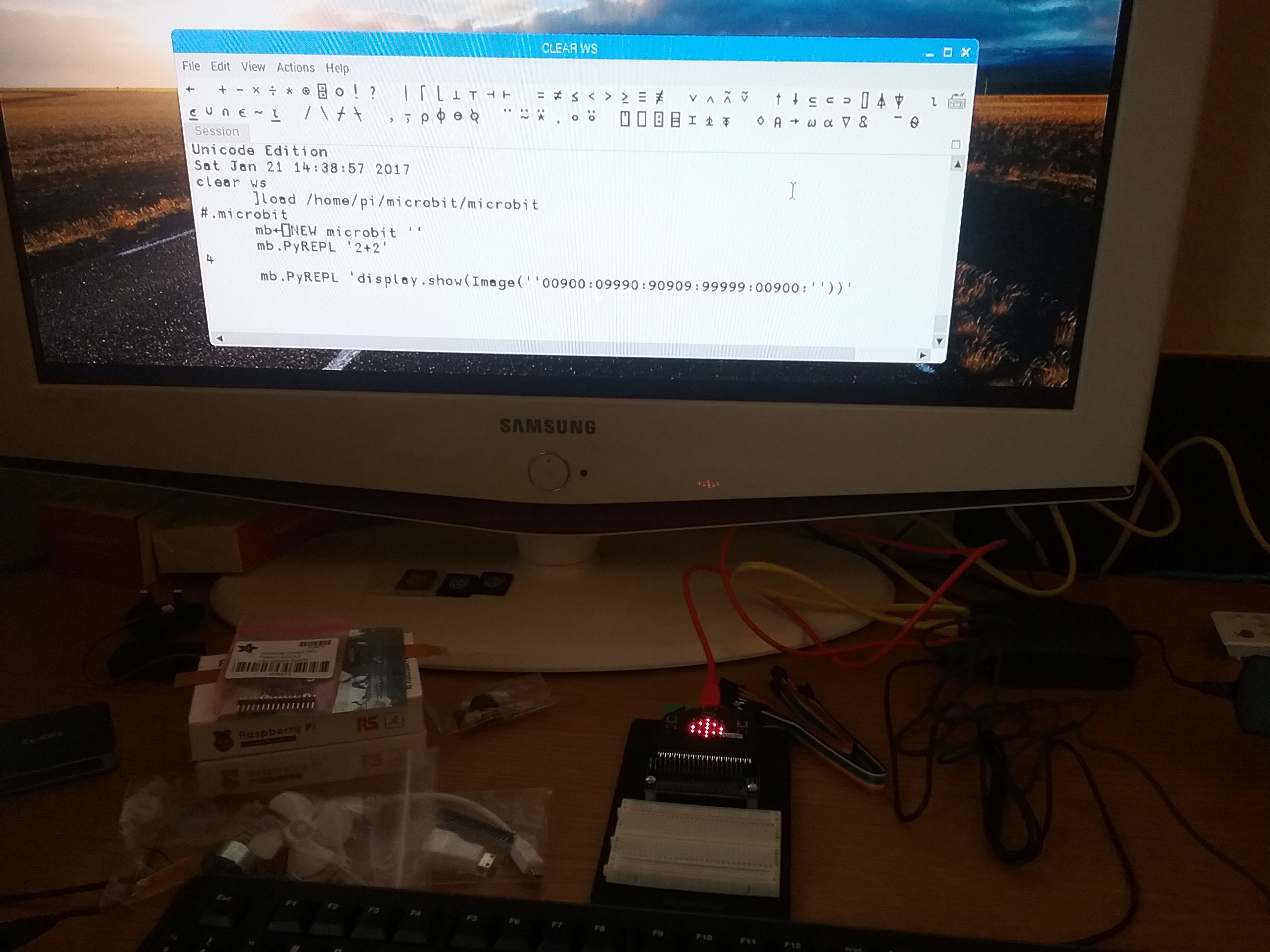
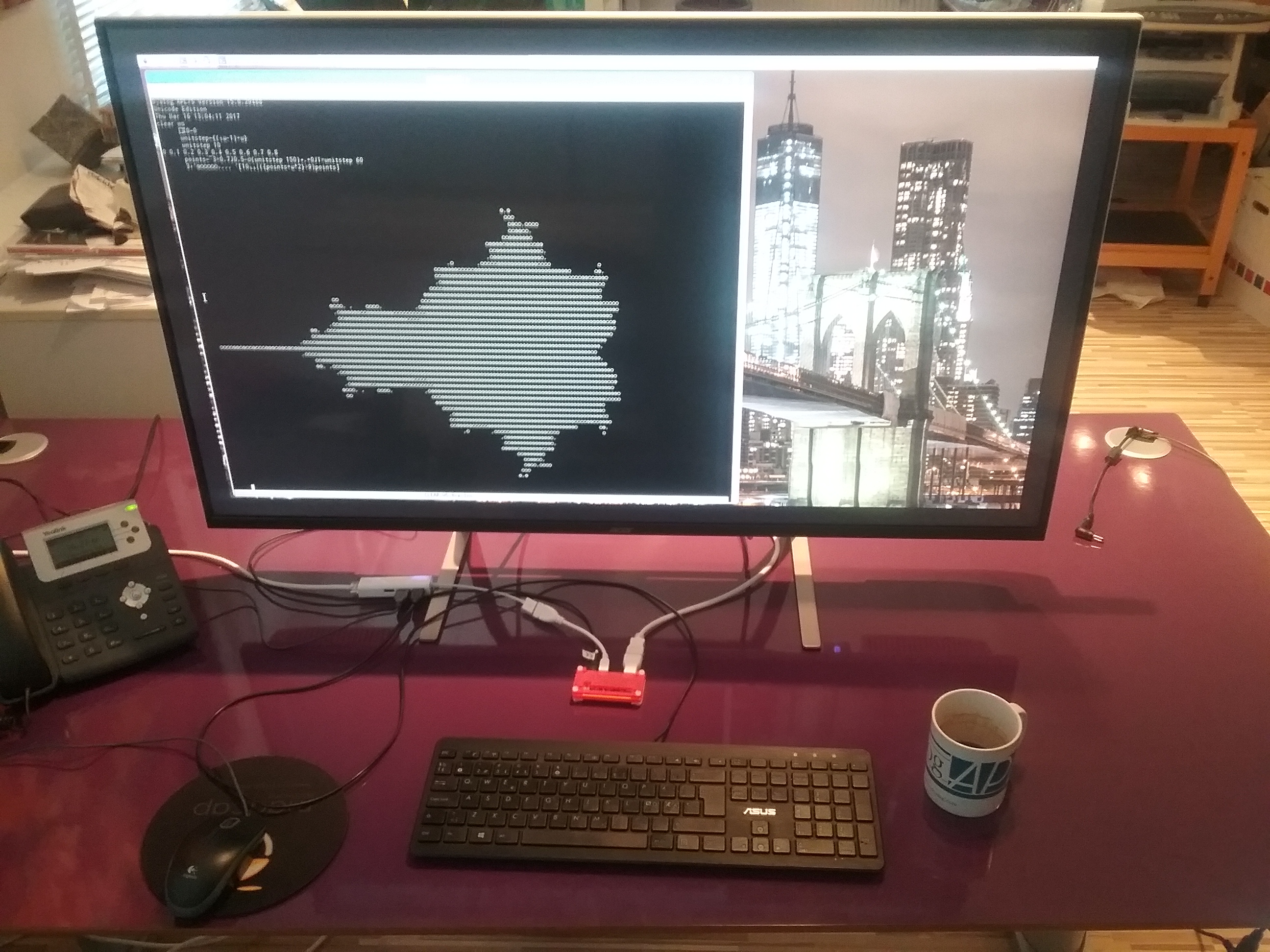
Finally, the last accessory I ordered for my Raspberry Pi Zero (that’s the little red thing behind my keyboard) has arrived – an Acer 43″ ET430K monitor. The Zero won’t quite drive this monitor at its maximum resolution of 3840×2160 pixels, but as you can see, you get enough real estate to do real graphics with “ASCII Art” (well, Unicode Art, anyway)!

Some readers will recognise the image as the famous Mandelbrot Set, named after the mathematician Benoit Mandelbrot, who studied fractals. According to Wikipedia a fractal is a mathematical set that exhibits a repeating pattern displayed at every scale – they are interesting because they produce patterns that are very similar to things we can see around us – both in living organisms and landscapes – they seem to be part of the fundamental fabric of the universe.

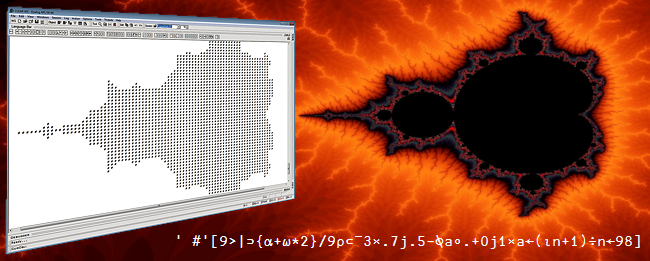
Fractals are are also interesting because they produce images of staggering beauty, as you can see on the pages linked to above and one of our rotating banner pages, where a one-line form of the APL expression which produced the image is embedded:

The colourful images of the Mandelbrot set are produced by looking at a selection of points in the complex plane. For each point c, start with a value of 0 for z, repeat the computation z = c + z², and colour the point according to the number of iterations required before the function becomes “unbounded in value”.

In APL, the function for each iteration can be expressed as {c+⍵*2}, where c is the point and ⍵ (the right argument of the function) is z (initially 0, and subsequently the result of the previous iteration):

      f←{c+⍵*2} ⍝ define the function
      c←1J1     ⍝ c is 1+i (above and to the right of the set)
      (f 0)(f f 0)(f f f 0)(f f f f 0) (f f f f f 0)
1J1 1J3 ¯7J7 1J¯97 ¯9407J¯193

If you are not familiar with complex numbers, those results may look a bit odd. While complex addition just requires adding the real and the imaginary parts independently, the result of multiplication of two complex numbers (a + bi) and (c + di) is defined as (ac-db) + (bc+ad)i. Geometrically, complex multiplication is a combined stretching and rotation operation.

Typing all those f’s gets a bit tedious, fortunately APL has a power operator ⍣, a second-order function that can be used to repeatedly apply a function. We can also compute the magnitude of the result number using |:

      (|(f⍣6)0)(|(f⍣7)0)
8.853E7 7.837E15

Let’s take a look at what happens if we choose a point inside the Mandelbrot set:

      c←0.1J0.1
      {|(f⍣⍵)0}¨ 1 2 3 4 5 6 7 8 9 10
0.1414 0.1562 0.1566 0.1552 0.1547 0.1546 0.1546 0.1546 0.1546 0.1546

Above, I used an anonymous function so I could pass the number of iterations in as a parameter, and use the each operator ¨ to generate all the results up to ten iterations. In this case, we can see that the magnitude of the result stabilises, which is why the point 0.1 + 0.1i is considered to be inside the Mandelbrot set.

Points which are just outside the set will require varying numbers of applications of f before the magnitude “explodes”, and if you colour points according to how many iterations are needed and pick interesting areas along the edge of the set, great beauty is revealed.

The above image is in the public domain and was created by Jonathan J. Dickau using ChaosPro 3.3 software, which was created by Martin Pfingstl.

Our next task is to create array of points in the complex plane. A helper function unitstep generates values between zero and 1 with a desired number of steps, so I can vary the resolution and size of the image. Using it, I can create two ranges, multiply one of them by i (0J1 in APL) and use an addition table (∘.+) to generate the array:

      ⎕io←0 ⍝ use index origin zero
      unitstep←{(⍳⍵+1)÷⍵}
      unitstep 6
0 0.1667 0.3333 0.5 0.6667 0.8333 1
      c←¯3 × 0.7J0.5 - (0J1×unitstep 6)∘.+unitstep 6
      c
¯2.1J¯1.5 ¯1.6J¯1.5 ¯1.1J¯1.5 ¯0.6J¯1.5 ¯0.1J¯1.5 0.4J¯1.5 0.9J¯1.5
¯2.1J¯1   ¯1.6J¯1   ¯1.1J¯1   ¯0.6J¯1   ¯0.1J¯1   0.4J¯1   0.9J¯1  
¯2.1J¯0.5 ¯1.6J¯0.5 ¯1.1J¯0.5 ¯0.6J¯0.5 ¯0.1J¯0.5 0.4J¯0.5 0.9J¯0.5
¯2.1      ¯1.6      ¯1.1      ¯0.6      ¯0.1      0.4      0.9     
¯2.1J00.5 ¯1.6J00.5 ¯1.1J00.5 ¯0.6J00.5 ¯0.1J00.5 0.4J00.5 0.9J00.5
¯2.1J01   ¯1.6J01   ¯1.1J01   ¯0.6J01   ¯0.1J01   0.4J01   0.9J01  
¯2.1J01.5 ¯1.6J01.5 ¯1.1J01.5 ¯0.6J01.5 ¯0.1J01.5 0.4J01.5 0.9J01.5

The result is subtracted from 0.7J0.5 (0.7 + 0.5i) to get the origin of the complex plane slightly off centre in the middle, and multiplied the whole thing by 3 to get a set of values that brackets the Mandelbrot set.

Note that APL expressions are typically rank and shape invariant, so our function f can be applied to the entire array without changes. Since our goal is only to produce ASCII art, we don’t need to count iterations, we can just compare the magnitude of the result with 9 to decide whether the point has escaped:

      9<|f 0
0 0 0 0 0 0 0
0 0 0 0 0 0 0
0 0 0 0 0 0 0
0 0 0 0 0 0 0
0 0 0 0 0 0 0
0 0 0 0 0 0 0
0 0 0 0 0 0 0
      9<|(f⍣3) 0 ⍝ Apply f 3 times
1 1 1 0 0 0 1
1 0 0 0 0 0 0
0 0 0 0 0 0 0
0 0 0 0 0 0 0
0 0 0 0 0 0 0
1 0 0 0 0 0 0
1 1 1 0 0 0 1

We can see that points around the edge start escaping after 3 iterations. Using an anonymous function again, we can observe more and more points escape, until we recognise the (very low resolution) outline of the Mandelbrot set:


      ]box on
      {((⍕⍵)@(⊂0 0))' #'[9>|(f⍣⍵)0]}¨2↓⍳9
┌───────┬───────┬───────┬───────┬───────┬───────┬───────┐
│2######│3  ### │4      │5      │6      │7      │8      │
│#######│ ######│   ### │    #  │    #  │    #  │    #  │
│#######│#######│ ##### │  #### │  #### │   ### │   ### │
│#######│#######│###### │ ##### │ ##### │ ##### │ ####  │
│#######│#######│ ##### │  #### │  #### │   ### │   ### │
│#######│ ######│   ### │    #  │    #  │    #  │    #  │
│#######│   ### │       │       │       │       │       │
└───────┴───────┴───────┴───────┴───────┴───────┴───────┘

The last example allowed me to sneak in a preview of the new “at” operator coming in Dyalog v16.0. It is a functional merge operator that I am using to insert the formatted right argument (the number of iterations) into position (0 0) of each matrix.

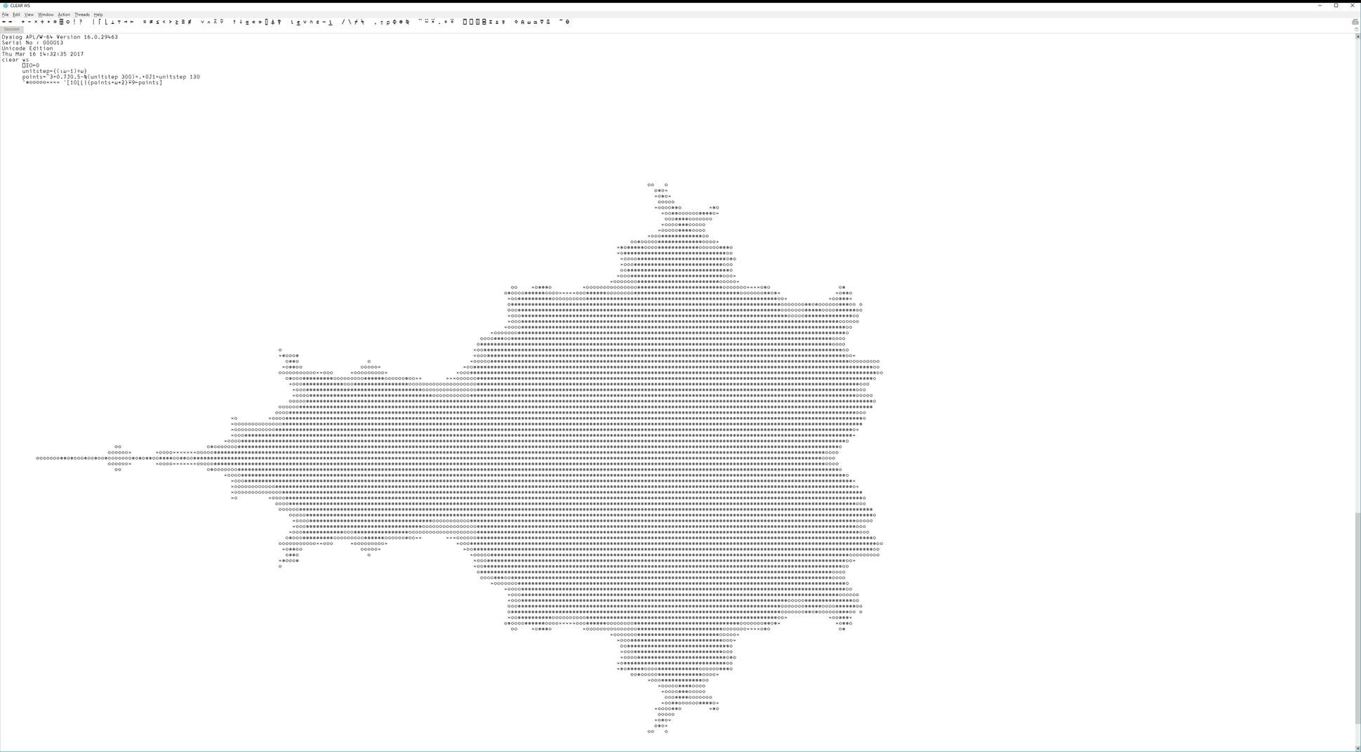
If I use our remote IDE (RIDE) on my Windows machine and connect to the Pi, I can have an APL session on the Pi with 3840×2160 resolution. In this example, I experimented with grey scale “colouring” the result by rounding down and capping the result at 10, and using the character ⍟ (darkest) for 0, ○ for 1-5, × for 6-9, and blank for points that “escaped”, by indexing into an array of ten characters:

      '⍟○○○○○×××× '[10⌊⌊|(f⍣9)c]

Who needs OpenGL?! (click on the image to enlarge)

Charting Reaction Times on the Raspberry Pi

Posted on March 10, 2017 by Morten Kromberg

Earlier this week I collected some reaction timer data on my Pi using the BBC micro:bit as an input device. I only produced an “ASCII art” chart at the time:

      times←ReactionTimer.Play
      times
251 305 294 415 338 298 294 251 378
      ReactionTimer.AsciiChart times
425| 
400|    * 
375|         *
350+ 
325|     * 
300|  * 
275|   *  ** 
250+ *      *

Retro is back in style – but of course I should point out that we can produce “proper” graphics using SharpPlot, a cross-platform graphics package that is included with Dyalog APL on all platforms. I’ve enhanced the ReactionTimer namespace with a function called SPHistogram. If you are using RIDE as the front end to APL on the Pi, this will render output from SharpPlot in a window:

    ReactionTimer.SPHistogram times

The original ASCII chart simply plotted the observations in the order that they occurred. Above, the shaded areas show how many observations there were in each bucket (2 between 250ms and 275ms, 3 between 275ms and 300ms, and so on). At the same time, the individual observations can be seen along the X axis as vertical red lines. It is a little unfortunate that, presumably due to some artifact of the timing process, the values 251 and 294 occur twice – and these lines are drawn on top of each other.

The example highlights one of the things that makes SharpPlot a bit special: We have overlaid a histogram showing the frequency of reactions in each bucket, and used a “scatterplot” to where the Y value is always 0, to mark the individual observations along the X axis.

     ∇ SPHistogram times;heading;renderHtml;sp;svg;z 
[1]   heading←'Reaction Times' 
[2]   renderHtml←3500⌶ ⍝ Render HTML in Window 
[3] 
[4]   :If 0=⎕NC'#.SharpPlot' ⋄ #.⎕CY'sharpplot.dws' ⋄ :EndIf
[5] 
[6]   sp←⎕NEW #.SharpPlot(432 250) 
[7]   sp.Heading←heading 
[8] 
[9]   ⍝ Draw histogram 
[10]  sp.ClassInterval←25 
[11]  sp.SetXTickMarks 25 
[12]  sp.HistogramStyle←#.HistogramStyles.SurfaceShading 
[13]  sp.SetFillStyles #.FillStyle.Opacity30 
[14]  sp.DrawHistogram⊂times 
[15] 
[16]  ⍝ Add observations using ScatterPlot 
[17]  sp.SetMarkers #.Marker.UpTick 
[18]  sp.SetPenWidths 1 
[19]  sp.SetMarkerScales 3 
[20]  sp.DrawScatterPlot(times×0)(times) 
[21] 
[22]  ⍝ Render SVG and display in window 
[23]  svg←sp.RenderSvg #.SvgMode.FixedAspect 
[24]  z←heading renderHtml svg 
     ∇

Hopefully the code is more or less self-explanatory, but if you’d like to learn more about SharpPlot there is excellent documentation at http://sharpplot.com. The documentation is actually written for C# users, but there is an illustration of how to translate the documentation to APL (and VB) at http://www.sharpplot.com/Languages.htm.

micro:bit Reaction Timer in APL on the Pi and BBC micro:bit

Posted on March 7, 2017 by Morten Kromberg

BBC micro:bit displaying a happy face

I have a bit of a cold today, so I decided that instead of hopping in an icy car and driving to the office in order to spend the day drinking coffee and answering e-mail, I should stay at home, turn up the radiators, make lots of tea (with honey!) and have some fun writing code on my Raspberry Pi! Can there be a better way to ensure a speedy recovery?

By the way, if you are already a user of Dyalog APL but you haven’t got a Pi yet, you should read The APLer’s Quick-start Guide to the Raspberry Pi, which Romilly Cocking completed a few days ago. This explains what your options are for buying hardware, and how to get going with a free copy of Dyalog APL. If you don’t read it now, your cold may be over before all the bits are delivered, so hurry up!

I wasn’t feeling THAT energetic this morning, so I decided to ease back into things by trying to replicate Romilly’s reaction timer, which is written in MicroPython. To begin with, I extended the microbit class that I developed for the Morse code display function with a few new methods to cover the API calls that allow me to check the state of the two buttons on each side of the micro:bit display (see the image above).

First, I added a method called is_true, which takes a MicroPython expression as an argument, evaluates it using the PyREPL function, and returns 0 or 1 depending on whether the expression returns False or True (and fails if it returns something else):

 ∇ r←is_true expr;t;z
 :Access Public
 r←1⊃t←'True' 'False'∊⊂z←PyREPL expr
 :If ~∨/t ⋄ ⎕←'True/False expected, got: ',z ⋄ ∘∘∘ ⋄ :EndIf
 ∇

This is a useful building block, which allows the simple construction of functions like was_pressed, which takes ‘a’ or ‘b’ as an argument and tells you whether the button in question has been pressed since you last asked:

∇ r←was_pressed button
 :Access Public
 r←is_true 'button_',button,'.was_pressed()' 
∇

Once this is done, writing the Play function in the ReactionTimer namespace is easy, you can find the rest of the code on GitHub. The APL version is different from the MicroPython version in that – once the user presses button B and stops the game – the reaction times (in milliseconds) are returned as an integer vector. So now we can have some fun with data!

In the spirit of the micro:bit, I thought I’d produce a low tech character based chart, trying to remember the skills that were start-of-the-art when I started using APL. The AsciiChart function in the ReactionTimer namespace takes a vector of timings as the right argument, and produces a chart:

      times←ReactionTimer.Play
      times
251 305 294 415 338 298 294 251 378
      ReactionTimer.AsciiChart times
425| 
400|    * 
375|         *
350+ 
325|     * 
300|  * 
275|   *  ** 
250+ *      *

The code (which is also on GitHub) is listed below. Because this is a pure function, I used the modern dfns style of function definition rather than the old style procedural form that I’ve used for the object oriented code. The function works by allocating each value to a bucket of the size defined by the variable scale. The fun part is the use of the outer product with equals (∘.=) between the list of buckets on the left (rb) and the scaled values on the right (⌊⍵÷scale) – and then using this Boolean array to index into a two-element character vector to produce the chart. The rest is scaling calculations and finally decorating with “tik marks”:

 AsciiChart←{
     scale←25 ⍝ size of each row
     tiks←4 ⍝ tik spacing
     (max min)←(⌈/ , ⌊/) ⍵ ⍝ maximum and minimum
     base←⌊min÷scale ⍝ round down to nearest scale unit
     rb←base+0,⍳⌈(max-min)÷scale ⍝ row base values
     r←' *'[1+rb∘.=⌊⍵÷scale] ⍝ our chart
     r←((≢rb)⍴'+',(tiks-1)⍴'|'),' ',r ⍝ add tiks
     r←(⍕⍪rb×scale),r ⍝ add base values
     ⊖r ⍝ low values last (humans!)
 }

Although I might be feeling better tomorrow, I expect to be back soon. I have a couple of plastic bags full of resistors, LEDs, potentiometers and cameras (yes, plural) that I have not opened yet!

Morse Code – Revisited using the BBC micro:bit

Posted on January 27, 2017 by Morten Kromberg

As mentioned last week, I have found a new way to provide a front end processor for my Pi, the BBC micro:bit. This week, I have started putting the new system through its paces: The microbit class in our GitHub repository has been beefed up to make it more resilient in the case where serial I/O is not initialised, or the MicroPython REPL is not running, and I have added a trivial Python program which can be used to intialise the REPL using the mu editor.

To test it all, I have revisited the Morse Code example, originally written to use GPIO support provided by Quick2Wire, to see if I could get it up and running with my new infrastructure. The micro:bit has a 5×5 LED display which makes the result a bit more impressive to look at:

The new code is significantly simpler than the original, for a couple of reasons:

Making calls to the micro:bit API via MicroPython is easier than using GPIO via a C library.
Version 15.0 of Dyalog APL contains new system functions for working with text files, so we no longer need the “Files” library, we can just use the built-in ⎕NGET function to read the contents of a file.

Raspberry APL Pi and Python on the micro:bit

Posted on January 24, 2017 by Morten Kromberg

A couple of years ago I spent many happy hours writing APL code to control robots which each embedded a Raspberry Pi. It was fun but it was a bumpy ride – my interest eventually faded when I discovered that it was just too difficult to make sense of raw accelerometer data, which I was hoping to use for precise navigation. After I managed to fry my MPU-9150, I decided to pursue other interests, as they say.

Recently, Romilly Cocking has been waxing lyrical about a number of new components which he thinks will make the whole experience more enjoyable – and I have decided to dive back in. So far, it has indeed been a very pleasant experience.

The Raspberry Pi Model 3

While I was away, the Raspberry Pi and the software available for it have come a VERY long way. The speed of a Pi 3 makes it a perfectly usable computer. I am writing this blog entry on the Pi using a standard Chromium browser. APL starts up immediately, using our new graphical IDE. It is quite simply amazing!

The BBC micro:bit and MicroPython

The first generation of APL-based robots used an Arduino to manage the motors and sensors because timing was too critical for the Pi to handle it. I spent some rather unhappy hours writing a control program in C, debugging that without any tools. You could not even do “printf debugging” to the serial port because that interfered with the timing so much that it stopped everything from working.

Romilly suggested I take a look at the micro:bit, and since I have been using an interactive REPL all my life, he suggested that I run MicroPython on it.

He was right, I’m loving it!

Getting Started

I purchased the Kitronik Inventors’s Kit for the micro:bit from Pimoroni, and quickly found videos on Youtube explaining how to assemble it. I installed the “mu” editor on my Pi and was immediately able to edit a simple Python program and run it on the micro:bit.

My next step was, of course, to create a little class to drive MicroPython from APL. This involves using serial I/O: when the micro:bit is attached to your Pi via USB it appears as a folder and as a serial (tty) device, typically /dev/ttyACM0. You can find my code in the APLPi/microbit GitHub repository.

If you clone the repository to /home/pi/microbit and start APL, you can make calls to the MicroPython repository along the lines of:

    ]load /home/pi/microbit/microbit    
    mb←⎕NEW microbit ''
    mb.PyREPL '2+2'
4

Using Python on the micro:bit to do maths isn’t that interesting when you have APL on the Pi; the exciting thing is that we can call the micro:bit Python API and access the hardware. My first experiment was to display my favourite APL symbol (Grade Up – aka Imperial Cruiser) in the built-in 5×5 LED display:

APL displaying an Imperial Cruiser on the micro:bit

Which of the Inventor’s Kit experiments would you like to see me do next?

Turning to a Heading with an MPU-9150

Posted on September 8, 2014 by Morten Kromberg

As the odour of fried electronics dissipates in the air, I’m unexpectedly afforded the opportunity to write this blog post a day or two earlier than planned. The on-board compass was exhibiting significant deviation, so I consulted my nephew Thorbjørn Christensen at DTU-Space. Thorbjørn makes a living designing magnetometers for space agencies around the world, and he suggested I use a ribbon cable to move the IMU away from the bot as a first step towards understanding the issue. He did warn me to be very careful when attaching it. I still don’t understand what I did wrong, but the evidence that I screwed up is pretty definitive: there are burn marks around every single connector and the IMU chip looks a bit soft in the middle. Most importantly, it no longer reports for duty on the Raspberry Pi’s I2C bus!

A fried IMU-9150 (click to enlarge)

The good news (apart from the fact that the Raspberry Pi, the Arduino and all other ‘bot components seem to have survived) is perhaps that, since I cannot play with the compass until I have a replacement, I found the time to write about where I am at the moment…and take some time out to work on my presentations for Dyalog ’14 (for those who managed to register before the user meeting in Eastbourne sold out, I still hope to do a ‘bot presentation on the evening of Tuesday September 23rd).

Introducing the MPU-9150

For the last few weeks, I have been using my “bot time” to play with the MPU-9150 breakout board that is attached to our ‘bot. The MPU-9150 is more or less identical to the 6050 that we were using earlier this summer to make gyro-controlled turns but also includes a magnetic compass, which will allow us to know the direction that we are heading in – making it a 9 degree of freedom inertial measurement unit, or “9-dof IMU” (9 = 3 gyro axes + 3 accelerometer axes + 3 compass axes).

RTIMULib

I was extremely happy to discover that Richard Barnett had shared his RTIMULib on GitHub. RTIMULib is a Linux library that produces “Kalman-filtered quaternion or Euler angle pose data” based on data from a 9-dof IMU. Jay Foad at Dyalog was quickly able to provide me with a couple of additional C functions designed to be easy to call from Dyalog APL. Jay’s fork of RTIMULib is also available on GitHub. Since we can assume that we are driving on a flat surface, I have just been using two items from the wealth of information provided by this library: the current rate of rotation and the current compass direction – in both cases around the vertical (or “z”) axis.

My First Compass-Controlled Rotation

Due to the fried IMU, I am unable to post a video recording; fortunately, at the moment where I toasted the chip, the Dyalog session output still contained output data from the last run of the function I am working on, which aims to provide smooth rotation to a selected compass heading. In the chart below, the red line tracks the speed of rotation and shows that the “smooth” part still needs work – the speed oscillates quite violently between 60 and 150 degrees per second. The blue line shows the number of degrees that the ‘bot still needs to turn to reach the desired heading. The dotted red line is slightly mislabeled: rather than acceleration, it actually shows the power applied to the motors via a digital-to-analog converter that accepts values between 0 and 255, producing between 0 and 5v of voltage for the DC motors:

Commentary:

From 0 to 0.4 seconds, we slowly increase power until we detect that rotation has started. We note the power setting required to start rotation.
0.4 to 0.7 (ish), we detect acceleration and hold the throttle steady (increasing it very slightly a couple of times when acceleration appears to stop).
0.7 to 1.1 seconds, cruise mode: whenever speed is above the target of 100 degrees/sec, we idle. When speed is below 100, we re-apply power at a level that was sufficient to start the rotation.
1.1 to 1.4 seconds: We are less than 30 degrees from target, and the target velocity and thus power is reduced proportional to the remaining distance (at 15 degrees, we are down to 50 deg/sec)
1.4 to 1.6 seconds: We detect that we rotated too far, and slam on the brakes, coming to a stop about 10 degrees from target.
1.6 to 2.3 seconds: since we are less than 10 degrees from target, we enter “step” mode, giving very brief bursts of power at “start rotation” level, idling, and watching the heading until we reach the goal.
2.4 seconds: We count the bursts and, after 10, we double the power setting to avoid getting bogged down (you cannot see the bursts in the chart, it only records the power level used for each one). A little more patience would have been good, this probably means we overshot by a bit.

The “Heading” Function

Achieving anything resembling smooth movement is still some way away, mostly due to the fact that motor response to a given input voltage varies enormously from motor to motor and between different applications to the same motor. The strategy described above is implemented by a function named “Heading”, which can be found in the file mpu9150.dyalog in the APLBot folder on GitHub. An obvious improvement would be to have the robot self-calibrate itself somehow and add a model of how fast rotation speeds up and slows down (based on, and constantly adjusted with, observed data), in order to dampen the oscillations. I intend to return to this when I have a new IMU (and my other user meeting presentations are under control).

This has turned out to be a lot harder than I imagined: suggestions are very welcome – please leave comments if you have a good idea!

The tool of thought for

software solutions

Contact Us

Category Archives: Raspberry Pi