Warning: The formula for “tolerated” comparison in this post is not correct for actual floating-point numbers. Do not use it! The follow-up post discusses how to compute the required value precisely in the presence of floating-point error.

Tolerant comparison is an important feature in making APL usable in the real world. But it’s also a lot slower than exact comparison. We think this tradeoff is well worth it (and of course, if you don’t want to make it, just set ⎕CT←0). But once in a while we can completely get rid of the slowdown! Added in Dyalog 17.0, along with vectorised comparison code so fast you might not even notice this change, is a cool technique that I call “tolerated comparison”. It works by turning a tolerant comparison with one argument fixed into an intolerant comparison by adjusting that fixed argument. So if you’re comparing one floating-point number to many of them, your code will run 30-40% faster than it would without this improvement.

Why tolerance?

Let’s take a trip to a slightly different APL.

      ⎕CT←0

A world in which tolerant comparison hasn’t been invented. Two things are equal when they’re the same.

      0.1 = 0.3-0.2
0
      {(0.1×⍵) = ⍵÷10} ⍳8
1 1 0 1 1 0 0 1

Okay, that’s a scary place. What happened?

The floating-point format can’t possibly represent every real number. Instead, there’s a carefully chosen set containing just shy of 2*64 numbers which can be expressed. For other numbers, we pick the closest available floating-point number. Usually this is a pretty accurate approximation. But once we perform arithmetic with a few of these values, we might go from “closest possible approximation” to “second-closest approximation” or even further away. The differences are still tiny, but when the same value—mathematically speaking—is computed in two different ways the results might be different numbers. Just barely different, but in a world without tolerant comparison that means they won’t be equal any more.

Tolerant comparison is an attempt to fix this. It’s not perfect, but it’s better in a lot of real-world situations. It makes = a useful function. The rule is that two values are equal when their difference is at most ⎕CT times the larger of their magnitudes. This is often called a “relative epsilon comparison” outside of the APL world.

Notation: To avoid confusion in the following text, I have used the APL symbols <≤=≥>≠ for intolerant comparisons, and the non-APL symbols ⋦≲≂≳⋧≉ to refer to APL’s tolerant comparisons which depend on ⎕CT. Watch out for a few quirks due to the scarcity of symbols to use: the actual APL primitives are denoted by non-APL characters, and the simpler symbol < “less-than” corresponds to the more complicated ⋦ “less-than and not approximately equal to”.

Tolerant comparisons

The famous formula for tolerant equality a≂b in terms of intolerant inequality (introduced here) is

(|a-b) ≤ ⎕CT×(|a)⌈(|b)

This allows for a little variation in the arguments, provided that neither one is zero. And it has some other nice properties, assuming ⎕CT≤1:

• It’s reflexive: a≂a for any number a.
• It’s symmetric in a and b: reversing them makes no difference in the result. This is because ⌈ and (|-) are symmetric functions.
• It scales linearly: multiplying both a and b by the same nonzero value (even a negative number) does not change the result.
• It’s convex in each variable: if a≂b and a≂d for some a, and c is between b and d, then a≂c.

In fact, tolerant equality as in APL is the only solution (or family of solutions, taking the ⎕CT parameter into account) to those constraints, other than the trivial one in which any two numbers are equal.

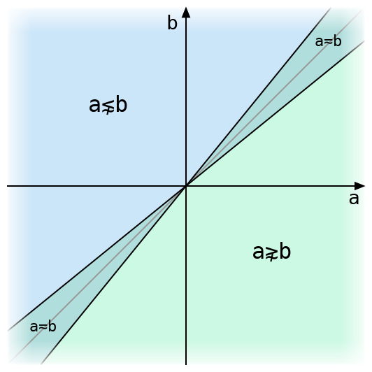
The above figure illustrates tolerant comparison of two real numbers. They are exactly equal only on the grey diagonal line, and tolerantly equal within the narrow strip around it. The diagram uses a much larger value for ⎕CT than Dyalog’s default of 1e¯14, or even its maximum allowed value of 2*¯32, either of which would make that strip invisible.

One way to define tolerant inequalities in terms of tolerant equality is to define, for instance, (a≲b) ≡ (a<b)∨(a≂b) using intolerant less-than and tolerant equality. But we’ll find it more useful to define ≲ and ≳ directly in terms of intolerant comparisons as with ≂. The formula for ≲ is:

(a-b) ≤ ⎕CT × 0⌈a⌈-b

and for ≳ we can use either (a≳b) ≡ (b≲a) or (a≳b) ≡ (-a)≲(-b) to obtain

(b-a) ≤ ⎕CT × 0⌈b⌈-a

or, negating both sides and swapping the inequality,

(a-b) ≥ ⎕CT × 0⌊a⌊-b

The 0⌈ term isn’t strictly necessary (as we’ll show later), but it helps avoid some confusion when a and b have different signs. Sometimes it’s used to speed up comparison by checking if a≤b intolerantly before performing any multiplication—if it is, the multiplication isn’t needed.

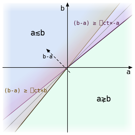
Above we can see how the equation for tolerant ≲ splits into two symmetrical half-formulas, each of which is just a little off from the exact inequality a≤b. The tolerant inequality accepts either of these conditions.

The region of tolerant equality is now the intersection of the regions for tolerant ≲ and ≳. That is:

(a≂b) ≡ (a≲b)∧(a≳b)

We’ll find this decomposition handy later on since tolerant inequalities are so much easier to work with.

Tolerating an inequality

What happens if we fix one side of the inequality? Here’s a diagram for a≲b with a dashed line drawn where b is equal to some fixed B and a varies.

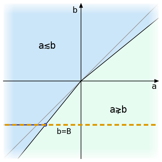
There’s only one place where the black line bounding the region where a≲b intersects the line b=B. The value of a at this intersection has an interesting property: when a is (exactly) less than or equal to that value, then it is tolerantly less than or equal to B. If we want to compare B to many other floating-point values, and we know the a coordinate of the intersection above, then we can skip all of the tolerant comparison arithmetic and just use exact comparison with that value!

Once we have a way to do this for ≲ all other inequalities will follow, since (a≳B) ≡ (-a)≲(-B) and (a⋧B) ≡ ~(a≲B).

Maybe you can figure out the value from the graphs above. But it’s also easy to find the value (and prove it works!) using a fact about the maximum function: for real numbers x, y, and z, x≤y⌈z is the same as (x≤y) ∨ (x≤z). One of the advantages of treating inequalities as functions like any other is that formulas like these are easy to manipulate. Here we go:

Start with the formula for tolerant inequality, writing q in place of ⎕CT.

(a-B) ≤ q × 0⌈a⌈-B

Distributing q× over ⌈, we have

(a-B) ≤ 0 ⌈ (q×a) ⌈ (-q×B)

and using (x≤y⌈z) ≡ ((x≤y) ∨ (x≤z)) twice (just like in the previous step, this can be thought of as distributing x≤ over three arguments of an associative function all at once), we can expand this formula to

((a-B) ≤ 0) ∨ ((a-B) ≤ q×a) ∨ ((a-B) ≤ -q×B)

which simplifies to

(a ≤ B) ∨ ((a×1-q) ≤ B) ∨ (a ≤ B×1-q)

or (here we need q<1, so that 1-q is positive; otherwise we’d have to reverse the middle inequality)

(a ≤ B) ∨ (a ≤ B÷1-q) ∨ (a ≤ B×1-q)

Recombining, we get

a  ≤  B ⌈ (B÷1-q) ⌈ (B×1-q)

So that’s our formula: now the tolerant equality is an intolerant equality, where the right side depends only on B!

Reading the signs

So we have a formula for a “tolerated” value b = B ⌈ (B÷1-q) ⌈ (B×1-q). When do the different possible maxima come into play?

• If B=0, then everything on the right is zero, and b=0.
• If B>0, then B×1-q is smaller than B, since q>0. But that means ÷1-q is larger than 1, and B÷1-q is larger than B. So b=B÷1-q.
• If B<0, then the all the inequalities that we got with B>0 are reversed. This means b=B×1-q.

Note that none of these cases depend on the branch b=B, even though the first one touches it. That means the definition of tolerant inequality would be the same even if we remove that branch. By working backwards through the above derivation we find that the initial 0⌈ has no effect, and we can remove it from the definition.

Equality

Tolerant equality obviously can’t be reduced to intolerant equality, since many values can be tolerantly equal to a number but only one is intolerantly equal to it. But recalling that (a≂b) ≡ (a≲b)∧(a≳b), we can express it as two intolerant inequalities: tolerate b for ≲ as above. Then tolerate it for ≳ (this always yields a value at least as large as the first). a is tolerantly equal to b if it lies between the two tolerated values.

This case is particularly important for the set functions ⍳∊∩∪~, which by definition use tolerant equality to match values in one argument to values in the other. If the non-principal argument (the one containing values to be looked up, like the right argument to ⍳) is short enough, then each element in it is looked up using a simple linear search through the principal argument. This means that one number at a time is compared to the entire principal argument (up to the first match found). So for floats we can get a substantial improvement by tolerating each element on the right before comparison.

Caution!

That was the easy part.

In this post we’ve been assuming that floating-point numbers behave like mathematical real numbers. Given that the whole reason tolerant comparison was introduced is that they don’t, maybe that wasn’t the best assumption.

The formulas B÷1-q and B×1-q for tolerated comparison are flawed: they produce values that differ slightly from the actual number that should be used in an intolerant equivalent to tolerant comparison. This is very dangerous: many programs could break if two values compare equal in one comparison but not in another! In the next post we’ll dive into the world of floating-point error analysis and find out how to get the right values. And we’ll discover that imperfect computation isn’t all bad when we find a faster alternative to a very slow floating-point division.

Follow