PQA

PQA is an acronym for Performance Quality Assurance. We developed PQA to answer the questions, which APL primitives have slowed down from one build of the Dyalog interpreter to the next, and by how much? Currently, PQA consists of 13,659 benchmarks divided into 136 groups.


4

The Graphs

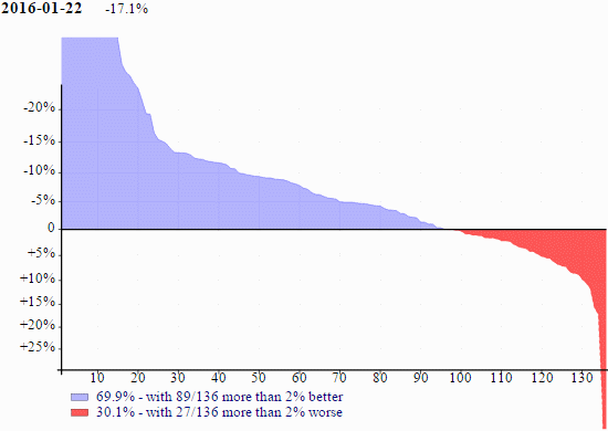
The graph above (and all other graphs in this article) plot the timing ratios between version 14.1 and the build of version 15.0 on 2016-01-22, the Windows 64-bit Unicode version. The data are the group geometric means. The horizontal axis are the groups sorted by the means. The vertical axis are logarithms of the means. The percent at the top (-17.1%) indicates that over all 136 groups, version 15.0 is 17.1% faster than version 14.1. The bottom of the graph indicates how many of the groups are faster (blue, 69.9%) and how many are more than 2% faster (89/136); and how many are slower (red, 30.1%) and how many are more than 2% slower (27/136).

For the graph above, the amount of blue is gratifying but the red is worrying. From past experience the more blue the better (of course) but any significant red is problematic; speed-ups will not excuse slow-downs.

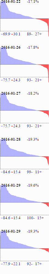
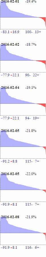
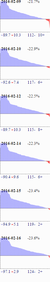
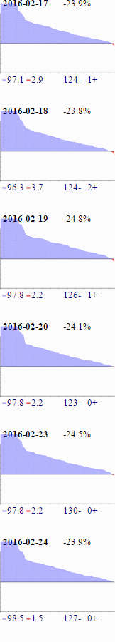
PQA is run nightly when a new build of version 15.0 is available. Each PQA run takes about 12.5 hours on a dedicated machine. The graphs from the past month’s runs are presented on the strip on the right; the first of them is a shrunken version of the big graph at the beginning of the article.

Challenges

About two years ago, investigations into a user report of an interpreter slow-down underscored for us a “feature” of modern computer systems: An APL primitive can run slower even though the C source is changed only in seemingly inconsequential ways and indeed even unchanged. Moreover, the variability in measurements frequently exceeded the difference in timings between the two builds, and it was very difficult to establish any kind of pattern. It got to the point where even colleagues were doubting us — how hard can it be to run a few benchmarks?

  • The system is very noisy.
  • Cache is king.
  • The CPU acts like an interpreter.
  • Branching (in machine code) is slow.
  • Instruction counts don’t tell all.
  • The number of combinations of APL primitives and argument types is enormous.

What can be done about it?

  • Developed PQA.
  • Run PQA on a dedicated machine.
  • Make the system as quiet as possible, then make it quieter than that. 🙂
  • Set the priority of the APL task to be High or Realtime.
  • The ⎕ai or ⎕ts clocks have insufficient resolution. Use QueryPerformanceCounteror equivalent. The QPC resolution varies but is typically around 0.5e¯6 seconds.
  • Run each benchmark expression enough times to consume a significant amount of time (50e¯3 seconds, say).
  • Repeat the previous step enough times to get a significant sample.

Despite all these, timing differences of less than 5% are not reliably reproducible.

Silver Bullets

Given the difficulties in obtaining accurate benchmarks and given the amount of time and energy required to investigate (phantom) slow-downs, there evolved among us the idea of “silver bullets”: We will actively work on speed-ups instead of waiting for slow-downs to bite.

The speed-ups to be worked on are chosen based on:

  • decades of experience in APL application development
  • decades of experience in APL design and implementation
  • APLMON snapshots provided by users
  • talking to users
  • interactions on the Dyalog Forums
  • running benchmarks on user applications
  • user presentations at Dyalog User Meetings
  • the speed-up is easy, while mindful of Einstein’s admonition against drilling lots of holes where the drilling is easy

We were gratified to receive reports from multiple users that their applications, without changes, sped up by more than 20% from 13.2 to 14.0. A user reported that using the key operator in 14.0 sped up a key part of their application by a factor of 17. Evidently some of the silver bullets found worthwhile targets.

We urge you, gentle reader, to send us APLMON snapshots of your applications, to improve the chance that future speed-ups will actually speed up your applications. APLMON is a profiling facility that indicates which APL primitives are used, how much they are used, the size and datatype of the arguments, and the proportion of the overall time of such usage. An APLMON snapshot preserves the secrecy of the application code.

We will talk about the new silver bullets for version 15.0 in another blog post. Watch this space.

Coverage

We look at benchmarks involving + as a dyadic function to give some idea of what’s being timed. There are 72 such expressions. Variables with the following names are involved:

      'xy'∘.,'bsildz'∘.,'0124'
┌───┬───┬───┬───┐
│xb0│xb1│xb2│xb4│
├───┼───┼───┼───┤
│xs0│xs1│xs2│xs4│
├───┼───┼───┼───┤
│xi0│xi1│xi2│xi4│
├───┼───┼───┼───┤
│xl0│xl1│xl2│xl4│
├───┼───┼───┼───┤
│xd0│xd1│xd2│xd4│
├───┼───┼───┼───┤
│xz0│xz1│xz2│xz4│
└───┴───┴───┴───┘
┌───┬───┬───┬───┐
│yb0│yb1│yb2│yb4│
├───┼───┼───┼───┤
│ys0│ys1│ys2│ys4│
├───┼───┼───┼───┤
│yi0│yi1│yi2│yi4│
├───┼───┼───┼───┤
│yl0│yl1│yl2│yl4│
├───┼───┼───┼───┤
│yd0│yd1│yd2│yd4│
├───┼───┼───┼───┤
│yz0│yz1│yz2│yz4│
└───┴───┴───┴───┘

x and y denote left or right argument; bsildz denote:

b
s
i
l
d
z
boolean
short integer
integer
long integer
double
complex
1 bit
1 byte
2 bytes
4 bytes
8 bytes
16 bytes

0124 denote the base-10 log of the vector lengths. (The lengths are 1, 10, 100, and 10,000.)

The bsil variables are added to the like-named variable with the same digit, thus:

xb0+yb0  xb0+ys0  xb0+yi0  xb0+yl0
xs0+yb0  xs0+ys0  xs0+yi0  xs0+yl0
xi0+yb0  xi0+ys0  xi0+yi0  xi0+yl0
xl0+yb0  xl0+ys0  xl0+yi0  xl0+yl0

xb1+yb1  xb1+ys1  xb1+yi1  xb1+yl1
xs1+yb1  xs1+ys1  xs1+yi1  xs1+yl1
...
xi4+yb4  xi4+ys4  xi4+yi4  xi1+yl4
xl4+yb4  xl4+ys4  xl4+yi4  xl4+yl4

There are the following 8 expressions to complete the list:

xd0+yd0  xd1+yd1  xd2+yd2  xd4+yd4
xz0+yz0  xz1+yz1  xz2+yz2  xz4+yz4

The idea is to measure the performance on small as well as large arguments, and on arguments with different datatypes, because (for all we know) different code can be involved in implementing the different combinations.

After looking at the expressions involving+, the wonder is not why there are as many as 13,600 benchmarks but why there are so few. If the same combinations are applied to other primitives then for inner product alone there should be 38,088 benchmarks. (23×23×72, 23 primitive scalar dyadic functions, 72 argument combinations.) The sharp-eyed reader may have noticed that the coverage for + already should include more combinations:

  xb0+yb1  xb0+yb2  xb0+yb4
  xb0+ys1  xb0+ys2  xb0+ys4
  xb0+yi1  xb0+yi2  xb0+yi4
  xb0+yl1  xb0+yl2  xb0+yl4
  ...
  xl0+yi1  xl0+yi2  xl0+yi4
  xl0+yl1  xl0+yl2  xl0+yl4 

We will be looking to fill in these gaps.
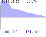
More on the Graphs

You should know that the PQA graphs shown here are atypical. The “blue mountain” is higher and wider than we are used to seeing, and it is unprecedented for a graph (the one for 2016-02-26) to have no red at all.

From version 15.0, the list of new silver bullets is somewhat longer than usual, but silver bullets usually only explain the blue peak. (Usually, speed-ups are implemented only if they offer a factor of 2 or greater improvement, typically achieved only on larger arguments.) What of the part from the “inflection point” around 30 and thence rightward into the red pit?

We believe the differences are due mainly to using a later release of the C compiler, Visual Studio 2015 in 15.0 vs. Visual Studio 2005 in 14.1. The new C compiler better exploits vector and parallel instructions, and that can make a dramatic difference in the performance of some APL primitives without any change to the source code. For example:

      x←?600 800⍴0
      y←?800 700⍴0
      cmpx 'x+.×y' ⍝ 15.0
1.54E¯1
      cmpx 'x+.×y' ⍝ 14.1
5.11E¯1

(Not all codings of inner product would benefit from these compiler techniques. The way Dyalog coded it does, though.)

Together with improvements for specific primitives such as +.× the new C compiler also provides a measurable general speed-up. Unfortunately, along with optimizations the new C compiler also comes with pessimizations. (Remember: speed-ups will not excuse slow-downs.) Some commonly and widely used C facilities and utilities did not perform as well as before. Your faithful Dyalog development team has been addressing these shortcomings and successfully working around them. Having a tool like PQA has been invaluable in the process.

It has been an … interesting month for PQA from 2016-01-22 to 2016-02-27. Now it’s onward to ameliorating the red under Linux and AIX.

Isolated Mandelbrot Set Explorer

mandelbrot-equation

It amazes me that an equation so simple can produce images so beautiful and complex.  I was first introduced to the Mandelbrot set by the August 1985 issue of Scientific American. Wikipedia says “The Mandelbrot set is the set of complex numbers ‘c’ for which the sequence ( c , c² + c , (c²+c)² + c , ((c²+c)²+c)² + c , (((c²+c)²+c)²+c)² + c , …) does not approach infinity.” This means that in the images below, the areas in black are points in the Mandelbrot set and the other point colors are determined by how quickly that point “zooms” off towards infinity. The links above give a deeper discussion on the Mandelbrot set – for this post I’d like to focus on how I was able to speed my Mandelbrot set explorer up using isolates.

Mandelbrot Set
I find I learn things more easily through application than abstraction. In 2006 I wanted to learn more about the built-in GUI features of Dyalog for Windows and the application I chose was a Mandelbrot set explorer. While the basic algorithm for calculating a point in the Mandelbrot set is fairly simple, a 640×480 pixel image could involve over 75 million calculations. As new versions of Dyalog are released, I try to experiment with any applicable new features and possibly incorporate them into the explorer. For instance, when complex numbers were introduced in Dyalog, I modified the explorer to use them.

Dyalog v14.0 introduced a prototype of a parallel computing feature called isolates that may one day be integrated into the interpreter. Isolates behave much like namespaces except that they run in their own process with their own copy of the interpreter. Each process can run on a separate processor, greatly improving performance. You can even set up isolate servers on other machines.

Mandelbrot set calculations are ideal candidates for parallelization as:

  • they’re CPU intensive
  • each pixel can be calculated independently of others
  • there are no side effects and no state to maintain

The core calculation is shown below. It takes the real and imaginary parameters for the top left corner, the height and width of the image and the increment along each dimension and uses those parameters to build a set of co-ordinates, then iterates to see how quickly each co-ordinate “escapes” the Mandelbrot set.

 ∇ r←real buildset_core imaginary;height;i_incr;top;width;r_incr;left;set;coord;inds;cnt;escaped
  ⍝ Calculate new Mandelbrot set - remember using origin 0 (⎕IO←0)
  ⍝ real and imaginary are the parameters of the space to calculate
  ⍝       real            imaginary
  ⍝ [0]   width           height            of the image
  ⍝ [1]   increment size  increment size    along each axis
  ⍝ [2]   top             left              coordinates

   (height i_incr top)←imaginary            ⍝ split imaginary argument parameters
   (width r_incr left)←real                 ⍝ split real argument parameters
   set←coord←,(0J1×top+i_incr×⍳height)∘.+(left+r_incr×⍳width) ⍝ create all points in the image
   inds←⍳≢r←(≢coord)⍴0                      ⍝ initialize the result and create vector of indices
   :For cnt :In 1↓⍳256                      ⍝ loop up to 255 times (the size of our color palette)
       escaped←4<coord×+coord               ⍝ mark those that have escaped the Mandelbrot set
       r[escaped/inds]←cnt                  ⍝ set their index in the color palette
       (inds coord)←(~escaped)∘/¨inds coord ⍝ keep those that have not yet escaped
       :If 0∊⍴inds ⋄ :Leave ⋄ :EndIf        ⍝ anything left to do?
       coord←set[inds]+×⍨coord              ⍝ the core Mandelbrot computation... z←(z*2)+c
   :EndFor
   r←(height,width)⍴r                       ⍝ reshape to image size
 ∇

So, what’s involved in using isolates to parallelize the explorer?  As it turns out, not much! First I )COPYed the isolate namespace from the isolate workspace distributed with Dyalog v14.0. I wanted to be able to select the number of processors to use, so I added a line to my init function to query how many processors are available:

 processors←1111⌶⍬ ⍝ query number of processors

Next I wrote a small function to initialize isolates for as many processors as were selected (2 or more). Notice that when creating the isolates, I copy buildset_core (from above) into each one:

 ∇ init_isolates processors
  ⍝ called upon initialization, or whenever user changes number of processors to use
   f.isomsg.Visible←1    ⍝ turn form's "Isolates initializing" message on
   {}isolate.Reset''     ⍝ reset the isolates
   {}isolate.Config'processors'processors ⍝ set the number of processors
   :If processors>1      ⍝ if using more than one processor
       ⍝ create the isolates, populating each one with buildset_core
       isolates←isolate.New¨processors⍴⎕NS'buildset_core'
   :EndIf
   f.isomsg.Visible←0    ⍝ turn the form message off
 ∇

Finally, I wrote a routine to share the work between the selected number of processors and assemble the results back together.

 ∇ r←size buildset rect;top;bottom;left;right;width;height;vert;horz;rows;incr;imaginary;real
  ⍝ Build new Mandelbrot Set using isolates if specified
  ⍝ rect is the top, bottom, left, and right
  ⍝ size is the height and width of the image
   (top bottom left right)←rect
   (height width)←size
   vert←bottom-top                             ⍝ vertical dimension
   horz←right-left                             ⍝ horizontal dimension
   rows←processors{¯2-/⌈⍵,⍨(⍳⍺)×⍵÷⍺}height     ⍝ divide image among processors (height=+/rows)
   incr←vert÷height                            ⍝ vertical increment
   imaginary←↓rows,incr,⍪top+incrׯ1↓0,+\rows  ⍝ imaginary arguments to buildset_core
   real←width,(horz÷width),left                ⍝ real arguments to buildset_core
   :If processors=1                            ⍝ if not using isolates
       r←real buildset_core⊃imaginary          ⍝ build the image here
   :Else
       r←⊃⍪/(⊂real)isolates.buildset_core imaginary ⍝ otherwise let the isolates to it
   :EndIf
 ∇

The images below depicts what happens with 4 processors. Each processor builds a slice of the image and the main task assembles them together.
Drawing1

So, how much faster is it?  Did my 8 processor Intel Core i7 speed things up by a factor of 8? No, but depending on where in the Mandelbrot set you explore, the speed is generally increased by at least a factor of 2 and sometimes as high as 5 or 6. I thought about why this might be and have a couple of ideas…

  • There’s overhead to receive and assemble the results from each isolate.
  • The overall time will be the maximum of the individual times; if one slice is in an area that requires more iterations, then the main task needs to wait for those results, even if the other slices have already finished. I could possibly show this by updating the individual slices as they become available. Maybe next time 🙂

What impressed me was that I could speed up my application significantly with about 20 lines of code and maybe an hour’s effort – most of which was spent tinkering to learn isolates. You can download the Mandelbrot set explorer from my GitHub repository.

Creating Shortcuts (Microsoft Windows)

At Dyalog, a developer not only needs access to all of the readily available editions of the interpreter but also to earlier versions that are no longer officially supported. On my Microsoft Windows Desktop I have a folder that contains a shortcut to my developer builds of all these interpreters.

I’ve recently suffered a complete failure of my C drive which, of course, contained my Windows desktop and all my shortcuts – which were lost.

The Dyalog interpreter exists in Classic and Unicode editions and 32 and 64 bit flavours…for versions from 12.0 to 14.1 this is a total of 28 interpreters. I couldn’t bring myself to create each of those 28 shortcuts by hand; let’s not even consider that if I were to build both debug and optimised binaries that would be 56 shortcuts!

Fortunately we have an old COM example (in the shortcut.dws workspace) which is shipped with the product. It’s a trivial exercise to call the supplied SHORTCUT function in one or more (ahem!) loops to create all the required shortcuts:

 Dyalogs;vers;chars;bits;location;v;c;b;dyalog;dir;name

 vers←'12.0.dss' '12.1.dss' '13.0.dss' '13.1.dss' '13.2.dss' '14.0.dss' 'trunk'
 chars←'classic' 'unicode'
 bits←'32' '64'

 ⎕NA'u shell32|SHGetFolderPath* u u u u >0T'
 location←'\Dyalog',⍨2⊃SHGetFolderPath 0 0 0 0 255

 :For v :In vers
     :For c :In chars
         :For b :In bits

             dir←'e:\obj\',v,'\2005\apl\win\',b,'\',c,'\winapi\dev\dbg'
             dyalog←dir,'\dyalog.exe'
             name←'.lnk',⍨location,'\',({v↓⍨('.dss'≡¯4↑v)/¯4}v),' ',b,' ',c

             name SHORTCUT dyalog dir'' 1('' 0)0 ''
         :End
     :End
 :End

shortcuts