Announcing the Beta Programme for Dyalog APL Version 18.2


I am very pleased to be able to announce the start of the Beta testing of the next release of Dyalog APL! As explained in June, we decided to delay the release of version 18.1 in order to take a closer look at some of the optimisations that had been implemented in 18.0 (and were therefore also present in 18.1).

Our analysis of the optimised code concluded that, due to the nature of many of the new algorithms involving modern vector instructions and code generated from templates, we need significantly more time to create tests that will cover absolutely all the different cases that have been implemented. As a result, we do not feel that it is in the best interests of our users to release v18.1 in its current form.

The good news is that the features of modern source code management systems, combined with our collection of regression tests, have allowed us to create a new version of Dyalog APL that contains all of the new features added to versions 18.0 and 18.1. This includes bug fixes made during these two development cycles, but not the optimisations that make us feel uncomfortable. To differentiate this version from the existing version 18.1, we have decided to call the new version 18.2.

Everyone who was signed up for the v18.1 beta programme should now be able to download v18.2 beta. If you are not signed up as a beta tester already but would like to help us with testing, please get in touch. Under Microsoft Windows, testing should be significantly simpler this year, as we have started producing Microsoft Patch files (MSP) as the delivery mechanism for updates – something I have personally been looking forward to since before I joined Dyalog Ltd!

Version 18.2 Performance

One unavoidable consequence of the above is that the performance of v18.2 is closer to that of v17.1 than to v18.0. Our own tests show that we have not been pushed ALL the way back to “square one”: v18.2 appears to be slightly faster than version 17.1. Once v18.2 has been delivered we will work on carefully re-implementing the most valuable optimisations that have been removed. We welcome your input on which primitives you think we should speed up first, so please participate in testing v18.2 and let us know what you think we should prioritise as we start work on version 19.0!

Recommendations regarding Version 18.0

Over the summer, only one additional defect related to performance optimisation was discovered and fixed. We are not currently aware of any outstanding defects in v18.0 caused by recent optimisations. Dyalog Ltd is committed to providing support for version 18.0 until the arrival of the 3rd release following it, in accordance with normal policy.

However, if you have not yet upgraded to v18.0, Dyalog Ltd strongly recommends remaining on your current version and moving directly to v18.2 when it is released. If all goes well, this will happen at the end of 2021 or very early in 2022. If you are already using v18.0, then we recommend that you make plans to start evaluating v18.2 and moving to it as soon as possible.

Conclusion – and Apology

We are painfully aware that the defects found in v18.0 and the resulting uncertainty have seriously inconvenienced some of our users, and I apologise for this. The root cause is the growth and rejuvenation of the Dyalog development team. Our original processes for quality assurance relied on years of tacit knowledge; when enthusiastic new team members break significant new ground, more explicit planning and QA processes are required to make sure that new approaches are safe and stable.

When we resume work on optimisations following the release of v18.2, this will be done according to new guidelines that require the process to begin with a careful risk/benefit analysis of any enhancement to primitive functions. We will do everything that we can to move forward in a way that will allow us all to eventually look back on the events of 2021 as a significant step towards a more capable and reliable development organisation and product.

After all, in another two years it will be time to celebrate 40 years of Dyalog APL!

News and Recommendations Regarding Dyalog Versions 17.1, 18.0 and 18.1

Background

Dyalog version 18.0 contained the largest number of optimised algorithms in the history of Dyalog APL. Unfortunately, since its release, we have found that our process for review and testing of optimisations was insufficient to cope with the quantity and nature of the optimisations. Many of the new algorithms had edge cases that escaped both the existing regression tests and the new tests that were written as part of development.

In August 2020, after the issues were reported following the release of Dyalog version 18.0, we issued a caution against the use of version 18.0 in production. We added significant additional testing during September and October, and subsequently lifted the caution in November. In April 2021, a user encountered an additional defect leading to incorrect results in a rare case of membership (), and in June a crash in an extremely rare case of “where” (monadic ). Since then, our own internal testing has found a defect in interval index (dyadic ).

Current Status

We have made patches available as defects have been detected and fixed, and “Issue 4” of version 18.0, made available to all users on 22 June 2021, includes fixes for all known issues with optimised code.

Download Dyalog version 18.0 Issue 4: Commercial users  Non-commercial users

At this time, we are executing two high priority projects, one aimed at increasing safety in the short term, the other at completely eliminating problematic optimisations within a few months:

  • We have further increased our internal testing of version 18.0, to verify the correctness of the optimisations that are still in the distributed product.
  • We are holding back the release of version 18.1, which was originally scheduled for release this month, while we remove most of the optimisations that went into version 18.0. We hope to release version 18.1 before the end of the 3rd Quarter of 2021, but will not let it out the door until we have complete confidence in this new version.

Recommendations

Dyalog Ltd recommends that users of Dyalog APL take the following action:

  • If you are using version 17.1 or earlier, plan to skip version 18.0 and upgrade directly to version 18.1 when it becomes available.
  • If you are using version 18.0, apply the latest patches or reinstall using Issue 4 when it becomes available. Continue to monitor our DSS e-mail broadcasts and apply patches quickly if we should find and fix any further issues that you think might impact your application. When version 18.1 becomes available, plan to upgrade to it at your earliest convenience.

Support for Versions 17.1 and 18.0

Considering this extraordinary situation, we have decided to extend support for version 17.1 for one additional release cycle. In other words, version 17.1 will be supported until we release the 4th subsequent version of Dyalog APL. Note that we are about to provide an updated version 17.1 installer (“Issue 3”) which collects all updates to version 17.1 since the original release.

Version 18.0 will be supported for the normal number of cycles, that is, until we release the 3rd following version. However, Dyalog Ltd recommends upgrading to version 18.1 as soon as it becomes available and you are able to schedule the upgrade.

Non-Commercial Versions

Given the nature of these defects, it is our intention to update our non-commercial distributions of version 18.0, although this process may lag behind the distribution of patches to clients paying for support by some weeks.

Conclusion

We apologise for the significant inconvenience that we know this is causing for some of you and thank you for your patience. We have made significant changes to our internal procedures regarding risk assessment, verification, and testing requirements for changes to existing primitive functions, to avoid a recurrence.

We do expect to re-apply those optimisations that we believe provide significant performance benefits to justify the risk of making changes over the next few releases, using new processes.

Sincerely,

Morten Kromberg
CTO, Dyalog Ltd.

Towards Improvements to Stencil

Background

The stencil operator was introduced in Dyalog version 16.0 in 2017. Recently we received some feedback (OK, complaints) that (a) stencil does padding which is unwanted sometimes and needs to be removed from the result and (b) stencil is too slow when it is not supported by special code.

First, stencil in cases supported by special code is much faster than when it is not. The special cases are as follows, from Dyalog ’17 Workshop SA3.

   {⍵}      {⊢⍵}      {,⍵}      {⊂⍵}
{+/,⍵}    {∧/,⍵}    {∨/,⍵}    {=/,⍵}    {≠/,⍵}  
    
{  +/,A×⍵}    {  +/⍪A×⍤2⊢⍵}
{C<+/,A×⍵}    {C<+/⍪A×⍤2⊢⍵}
C:  a single number or variable whose value is a single number
A:  a variable whose value is a rank-2 or 3 array
The comparison can be < ≤ ≥ > = ≠
odd window size; movement 1; matrix argument
 

You can test whether a particular case is supported by using a circumlocution to defeat the special case recognizer.

   )copy dfns cmpx

   cmpx '{⍵}⌺3 5⊢y' '{⊢⊢⍵}⌺3 5⊢y' ⊣ y←?100 200⍴0
  {⍵}⌺3 5⊢x   → 4.22E¯4 |      0%                               
  {⊢⊢⍵}⌺3 5⊢x → 5.31E¯2 | +12477% ⎕⎕⎕⎕⎕⎕⎕⎕⎕⎕⎕⎕⎕⎕⎕⎕⎕⎕⎕⎕⎕⎕⎕⎕⎕⎕⎕⎕⎕⎕

   cmpx '{⌽⍵}⌺3 5⊢y' '{⊢⊢⌽⍵}⌺3 5⊢y'
  {⌽⍵}⌺3 5⊢y   → 2.17E¯1 |  0% ⎕⎕⎕⎕⎕⎕⎕⎕⎕⎕⎕⎕⎕⎕⎕⎕⎕⎕⎕⎕⎕⎕⎕⎕⎕⎕⎕⎕⎕⎕
  {⊢⊢⌽⍵}⌺3 5⊢y → 2.21E¯1 | +1% ⎕⎕⎕⎕⎕⎕⎕⎕⎕⎕⎕⎕⎕⎕⎕⎕⎕⎕⎕⎕⎕⎕⎕⎕⎕⎕⎕⎕⎕⎕

If the timings are the same then there is no special code.

Padding and performance improvements will take a lot of work. For example, for padding (i.e. the treatment of cells at the edge of the universe) multiple options are possible: no padding, padding, wrap from opposite edge, etc. While working on these improvements I hit upon the idea of writing a stencil function which produces the stencil cells. It only works with no padding and only for movements of 1 (which I understand are common cases), but turns out to be an interesting study.

A Stencil Function

⍺ stencell ⍵ produces the stencil cells of size from  , and is equivalent to {⍵}⌺⍺⊢⍵ after the padded cells are removed.

stencell←{
  ⎕io←0                 ⍝ ⎕io delenda est!
  s←(≢⍺)↑⍴⍵
  f←1+s-⍺               ⍝ frame AKA outer shape
  m←⊖×⍀⊖1↓s,1           ⍝ multiplier for each axis
  i←⊃∘.+⌿(m,m)×⍳¨f,⍺    ⍝ indices
  (⊂i) ⌷ ⍵ ⍴⍨ (×⌿(≢⍺)↑⍴⍵),(≢⍺)↓⍴⍵
}

For example, stencell is applied to x with cell shape 3 5 .

   ⊢ x←6 10⍴⍳60                    ⍝ (a)
 0  1  2  3  4  5  6  7  8  9
10 11 12 13 14 15 16 17 18 19
20 21 22 23 24 25 26 27 28 29
30 31 32 33 34 35 36 37 38 39
40 41 42 43 44 45 46 47 48 49
50 51 52 53 54 55 56 57 58 59

   c←3 5 stencell x                ⍝ (b)
   ⍴c
4 6 3 5

   c ≡ 1 2 ↓ ¯1 ¯2 ↓ {⍵}⌺3 5 ⊢x    ⍝ (c)
1

   ⊢ e←⊂⍤2 ⊢c                      ⍝ (d)
┌──────────────┬──────────────┬──────────────┬──────────────┬──────────────┬──────────────┐
│ 0  1  2  3  4│ 1  2  3  4  5│ 2  3  4  5  6│ 3  4  5  6  7│ 4  5  6  7  8│ 5  6  7  8  9│
│10 11 12 13 14│11 12 13 14 15│12 13 14 15 16│13 14 15 16 17│14 15 16 17 18│15 16 17 18 19│
│20 21 22 23 24│21 22 23 24 25│22 23 24 25 26│23 24 25 26 27│24 25 26 27 28│25 26 27 28 29│
├──────────────┼──────────────┼──────────────┼──────────────┼──────────────┼──────────────┤
│10 11 12 13 14│11 12 13 14 15│12 13 14 15 16│13 14 15 16 17│14 15 16 17 18│15 16 17 18 19│
│20 21 22 23 24│21 22 23 24 25│22 23 24 25 26│23 24 25 26 27│24 25 26 27 28│25 26 27 28 29│
│30 31 32 33 34│31 32 33 34 35│32 33 34 35 36│33 34 35 36 37│34 35 36 37 38│35 36 37 38 39│
├──────────────┼──────────────┼──────────────┼──────────────┼──────────────┼──────────────┤
│20 21 22 23 24│21 22 23 24 25│22 23 24 25 26│23 24 25 26 27│24 25 26 27 28│25 26 27 28 29│
│30 31 32 33 34│31 32 33 34 35│32 33 34 35 36│33 34 35 36 37│34 35 36 37 38│35 36 37 38 39│
│40 41 42 43 44│41 42 43 44 45│42 43 44 45 46│43 44 45 46 47│44 45 46 47 48│45 46 47 48 49│
├──────────────┼──────────────┼──────────────┼──────────────┼──────────────┼──────────────┤
│30 31 32 33 34│31 32 33 34 35│32 33 34 35 36│33 34 35 36 37│34 35 36 37 38│35 36 37 38 39│
│40 41 42 43 44│41 42 43 44 45│42 43 44 45 46│43 44 45 46 47│44 45 46 47 48│45 46 47 48 49│
│50 51 52 53 54│51 52 53 54 55│52 53 54 55 56│53 54 55 56 57│54 55 56 57 58│55 56 57 58 59│
└──────────────┴──────────────┴──────────────┴──────────────┴──────────────┴──────────────┘

    ∪¨ ,¨ e-⍬⍴e                    ⍝ (e)
┌──┬──┬──┬──┬──┬──┐
│0 │1 │2 │3 │4 │5 │
├──┼──┼──┼──┼──┼──┤
│10│11│12│13│14│15│
├──┼──┼──┼──┼──┼──┤
│20│21│22│23│24│25│
├──┼──┼──┼──┼──┼──┤
│30│31│32│33│34│35│
└──┴──┴──┴──┴──┴──┘
(a)  The matrix x is chosen to make stencil results easier to understand.
(b) stencell is applied to x with cell shape 3 5 .
(c) The result of stencell is the same as that for {⍵}⌺ after cells with padding are dropped.
(d) Enclose the matrices in c (the cells) to make the display more compact and easier to understand.
(e) Subsequent discussion is based on the observation that each cell is some scalar integer added to the first cell.

Indices

The key expression in the computation is

   ⊃∘.+⌿(m,m)×⍳¨f,⍺ 

where

   m:  10 1;  multiplier for each axis
   f:  4 6;  multiplier for each axis
   ⍺:  3 5;  multiplier for each axis
 

We discuss a more verbose but equivalent version of this expression,

   (⊃∘.+⌿m×⍳¨f)∘.+(⊃∘.+⌿m×⍳¨⍺)

and in particular the right half, ⊃∘.+⌿m×⍳¨⍺ , which produces the first cell.

   ⍳⍺               ⍝ ⍳3 5
┌───┬───┬───┬───┬───┐
│0 0│0 1│0 2│0 3│0 4│
├───┼───┼───┼───┼───┤
│1 0│1 1│1 2│1 3│1 4│
├───┼───┼───┼───┼───┤
│2 0│2 1│2 2│2 3│2 4│
└───┴───┴───┴───┴───┘
   (⍴⍵)∘⊥¨⍳⍺        ⍝ 6 10∘⊥¨ ⍳3 5
 0  1  2  3  4
10 11 12 13 14
20 21 22 23 24

Alternatively, this last result obtains by multiplying by m the corresponding indices for each axis, where an element of m is the increment for a unit in an axis. That is, m←⊖×⍀⊖1↓s,1 where s←(≢⍺)↑⍴⍵ is a prefix of the shape of  . The multipliers are with respect to the argument because the indices are required to be with respect to the argument  .

   ⍳¨⍺              ⍝ ⍳¨3 5
┌─────┬─────────┐
│0 1 2│0 1 2 3 4│
└─────┴─────────┘
   m×⍳¨⍺            ⍝ 10 1×⍳¨3 5
┌───────┬─────────┐
│0 10 20│0 1 2 3 4│
└───────┴─────────┘
   ∘.+⌿ m×⍳¨⍺       ⍝ ∘.+⌿ 10 1×⍳¨3 5
┌──────────────┐
│ 0  1  2  3  4│
│10 11 12 13 14│
│20 21 22 23 24│
└──────────────┘
   ((⍴⍵)∘⊥¨⍳⍺) ≡ ⊃∘.+⌿m×⍳¨⍺
1

This alternative computation is more efficient because it avoids creating and working on lots of small nested vectors and because the intermediate results for ∘.+⌿ grows fast from one to the next (i.e., O(⍟n) iterations in the main loop).

The left half, ⊃∘.+⌿m×⍳¨f , is similar, and computes the necessary scalar integers to be added to the result of the right half.

   ⊃ ∘.+⌿ m×⍳¨f     ⍝ ⊃ ∘.+⌿ 10 1×⍳¨4 6
 0  1  2  3  4  5
10 11 12 13 14 15
20 21 22 23 24 25
30 31 32 33 34 35

The shorter expression derives from the more verbose one by some simple algebra.

(⊃∘.+⌿m×⍳¨f)∘.+(⊃∘.+⌿m×⍳¨⍺)    ⍝ verbose version
⊃∘.+⌿(m×⍳¨f),m×⍳¨⍺             ⍝ ∘.+ is associative
⊃∘.+⌿(m,m)×(⍳¨f),⍳¨⍺           ⍝ m× distributes over ,
⊃∘.+⌿(m,m)×⍳¨f,⍺               ⍝ ⍳¨ distributes over ,

I am actually disappointed that the shorter expression was found ☺; it would have been amusing to have a non-contrived and short expression with three uses of ∘.+ .

Cells

Having the indices i in hand, the stencil cells obtain by indexing into an appropriate reshape or ravel of the right argument  . In general, the expression is

   (⊂i) ⌷ ⍵ ⍴⍨ (×/(≢⍺)↑⍴⍵),(≢⍺)↓⍴⍵

specifies the cell shape. If (≢⍺)=≢⍴⍵ , that is, if a length is specified for each axis of  , the expression is equivalent to (⊂i)⌷,⍵ or (,⍵)[i] ; if (≢⍺)<≢⍴⍵ , that is, if there are some trailing unstencilled axes, the expression is equivalent to (,[⍳≢⍺]⍵)[i;…;] (the leading ≢⍺ axes are ravelled) or ↑(,⊂⍤((≢⍴⍵)-≢⍺)⊢⍵)[i] (as if the trailing axes were shielded from indexing). The general expression covers both cases.

Application

stencell makes it possible to workaround current shortcomings in . The alternative approach is to use stencell to get all the stencil cells, all at once, and then work on the cells using  , +.× , and
other efficient primitives.

The following example is from Aaron Hsu. In the original problem the size of x is 512 512 64 .

   K←?64 3 3 64⍴0
   x←?256 256 64⍴0

   t←1 1↓¯1 ¯1↓{+/⍪K×⍤3⊢⍵}⌺3 3⊢x
   ⍴t
256 256 64

   cmpx '1 1↓¯1 ¯1↓{+/⍪K×⍤3⊢⍵}⌺3 3⊢x'
6.76E0 

The computation is slow because the cells are rank-3, not supported by special code. Aaron then devised a significant speed-up using a simpler left operand to create the ravels of the cells (but still no special code):

   t ≡ (1 1↓¯1 ¯1↓{,⍵}⌺3 3⊢x)+.×⍉⍪K
1
   cmpx '(1 1↓¯1 ¯1↓{,⍵}⌺3 3⊢x)+.×⍉⍪K'
1.67E0 

Use of stencell would improve the performance a bit further:

   t ≡ (,⍤3 ⊢3 3 stencell x)+.×⍉⍪K
1
   cmpx '(,⍤3 ⊢3 3 stencell x)+.×⍉⍪K'
1.09E0 

   cmpx '3 3 stencell x'
6.10E¯2

The last timing shows that the stencell computation is 6% (6.10e¯2÷1.09e0) of the total time.

Materializing all the cells does take more space than if the computation is incorporated in the left operand of  , and is practicable only if the workspace sufficiently large.

   )copy dfns wsreq

   wsreq '1 1↓¯1 ¯1↓{+/⍪K×⍤3⊢⍵}⌺3 3⊢x'
110649900
   wsreq '(1 1↓¯1 ¯1↓{,⍵}⌺3 3⊢x)+.×⍉⍪K'
647815900
   wsreq '(,⍤3 ⊢3 3 stencell x)+.×⍉⍪K'
333462260

Performance

stencell is competitive with {⍵}⌺ on matrices, where it is supported by special code written in C, and is faster when there is no special code. The benchmarks are done on a larger argument to reduce the effects of padding/unpadding done in {⍵}⌺ .

   y2←?200 300⍴0
          
   cmpx '3 5 stencell y2' '1 2↓¯1 ¯2↓{⍵}⌺3 5⊢y2' 
  3 5 stencell y      → 1.85E¯3 |   0% ⎕⎕⎕⎕⎕⎕⎕⎕⎕⎕⎕⎕⎕⎕⎕⎕⎕⎕⎕           
  1 2↓¯1 ¯2↓{⍵}⌺3 5⊢y → 2.91E¯3 | +57% ⎕⎕⎕⎕⎕⎕⎕⎕⎕⎕⎕⎕⎕⎕⎕⎕⎕⎕⎕⎕⎕⎕⎕⎕⎕⎕⎕⎕⎕⎕

   cmpx '3 5 stencell y' '{⍵}⌺3 5⊢y' 
  3 5 stencell y → 1.85E¯3 |   0% ⎕⎕⎕⎕⎕⎕⎕⎕⎕⎕⎕⎕⎕⎕⎕⎕⎕⎕⎕⎕⎕⎕⎕⎕⎕⎕⎕⎕⎕⎕
* {⍵}⌺3 5⊢y      → 1.04E¯3 | -45% ⎕⎕⎕⎕⎕⎕⎕⎕⎕⎕⎕⎕⎕⎕⎕⎕⎕             

   y3←?200 300 64⍴0

   cmpx '3 5 stencell y3' '1 2↓¯1 ¯2↓{⍵}⌺3 5⊢y3' 
  3 5 stencell y3      → 8.90E¯2 |    0% ⎕⎕⎕                           
  1 2↓¯1 ¯2↓{⍵}⌺3 5⊢y3 → 7.78E¯1 | +773% ⎕⎕⎕⎕⎕⎕⎕⎕⎕⎕⎕⎕⎕⎕⎕⎕⎕⎕⎕⎕⎕⎕⎕⎕⎕⎕⎕⎕⎕⎕

   cmpx '3 5 stencell y3' '{⍵}⌺3 5⊢y3' 
  3 5 stencell y3 → 9.38E¯2 |    0% ⎕⎕⎕⎕⎕⎕⎕⎕                      
* {⍵}⌺3 5⊢y3      → 3.34E¯1 | +256% ⎕⎕⎕⎕⎕⎕⎕⎕⎕⎕⎕⎕⎕⎕⎕⎕⎕⎕⎕⎕⎕⎕⎕⎕⎕⎕⎕⎕⎕⎕

There is an interesting question of whether the shorter version of the key computation (in the Indices section above) is faster than the more verbose version.

   m←10 1 ⋄ f←4 6 ⋄ a←3 5

   cmpx '⊃∘.+⌿(m,m)×⍳¨f,a' '(⊃∘.+⌿m×⍳¨f)∘.+(⊃∘.+⌿m×⍳¨a)'
  ⊃∘.+⌿(m,m)×⍳¨f,a            → 3.75E¯6 |   0% ⎕⎕⎕⎕⎕⎕⎕⎕⎕⎕⎕⎕⎕⎕⎕⎕⎕⎕⎕
  (⊃∘.+⌿m×⍳¨f)∘.+(⊃∘.+⌿m×⍳¨a) → 5.20E¯6 | +38% ⎕⎕⎕⎕⎕⎕⎕⎕⎕⎕⎕⎕⎕⎕⎕⎕⎕⎕⎕⎕⎕⎕⎕⎕⎕⎕

In this case, it is faster, and I expect it will be faster for cases which arise in stencil calculations, where the argument size is larger than the cell size. But it is easy to think of arguments where ∘.+⌿ is slower than ∘.+ done with a different grouping:

   cmpx '((⍳0)∘.+⍳100)∘.+⍳200' '(⍳0)∘.+((⍳100)∘.+⍳200)' '⊃∘.+/⍳¨0 100 200'
  ((⍳0)∘.+⍳100)∘.+⍳200   → 7.86E¯7 |     0% ⎕⎕                            
  (⍳0)∘.+((⍳100)∘.+⍳200) → 1.05E¯5 | +1234% ⎕⎕⎕⎕⎕⎕⎕⎕⎕⎕⎕⎕⎕⎕⎕⎕⎕⎕⎕⎕⎕⎕⎕⎕⎕⎕⎕⎕  
  ⊃∘.+/⍳¨0 100 200       → 1.11E¯5 | +1310% ⎕⎕⎕⎕⎕⎕⎕⎕⎕⎕⎕⎕⎕⎕⎕⎕⎕⎕⎕⎕⎕⎕⎕⎕⎕⎕⎕⎕⎕⎕

This question will be explored further in a later post.

Tolerated Comparison, Part 2

This post might be more difficult than our usual fare. You won’t find any interesting APL coding insights here—instead we’ll be focused on the tricky topic of floating-point error analysis. If that’s not your thing, feel free to skip this one! Although if you plan to use tolerated comparison in a real application, you really do need to know this stuff.

In Tolerated Comparison, Part 1, I discussed the structure of tolerant inequality with one argument fixed, and showed that

  • For any real number B, there’s another number b so that a number is tolerantly less than or equal to B if and only if it is intolerantly less than or equal to b.
  • This number is equal to B÷1-⎕CT when B<0, and B×1-⎕CT otherwise.

But these results were proven only for mathematical real numbers, which have many properties among which is the complete inability to be implemented in a silicon chip. To actually apply the technique in Dyalog APL, we must know that it works for IEEE floats like Dyalog uses (we have not implemented tolerated comparison for the decimal floating point numbers used when ⎕FR is 1287, and there are serious concerns regarding precision which might make it impossible to tolerate values efficiently).

Why should we care if a tolerated value is off by one or a few units in the last place? It’s certainly unlikely to cause widespread chaos. But we think programmers should be able to expect, for instance, that after setting i←v⍳x it is always safe to assume that v[i]=x. A language that behaves otherwise can easily cause “impossible” bugs in programs that are provably correct according to Dyalog’s specification. And finding a value that lies just on the boundary of equality with x is not as obscure an issue as it may appear. With the default value ⎕CT←1E¯14, there are at most about 180 numbers which are tolerantly equal to a typical floating-point number x. So it’s not much of a stretch to think that a program which handles a lot of similar values will eventually run into a problem with an inaccurate version of tolerated equality. And this is a really scary problem to debug—even the slightest difference in the values used would make it disappear, frustrating any efforts to track down the cause. We’ve dealt with tolerant comparison issues in the past and this kind of problem is certainly not something we want to stumble on in the future.

On to floating-point numbers. I’m afraid this is not a primer on the subject, although I can point any interested readers to the excellent What Every Computer Scientist Should Know About Floating-Point Arithmetic. In brief, Dyalog’s floating-point numbers use 64 bits to represent a particular set of real numbers chosen to cover many orders of magnitude and to satisfy some nice mathematical properties. We need to know only a surprisingly small number of things about these numbers, though—see the short list below. Here we consider only normal numbers, and not denormal numbers, which appear at extremely small magnitudes. The important result of this post is still valid for denormal numbers, which have higher tolerance for error than normal numbers, but we will not demonstrate this detail here.

Definitions: In the discussion below, q is used as a short name for the value ⎕CT. Unless stated otherwise, formulas below are to be interpreted not as floating-point calculations but as mathematical expressions—there is no rounding and all comparisons in formulas are intolerant. Evaluation order follows APL except that = is used as in mathematics: it has lower precedence and can be used multiple times in chains to show that many values are all equal to each other. The word “error” indicates absolute error, that is, the absolute distance of a computed value from some desired value. The value ulp (from “Unit in the Last Place”) is used to indicate what some might denote ULP(1), the distance from 1 to the next higher floating point number. It is equal to 2*¯52, and it is an upper bound on the error between two adjacent normal floating-point numbers divided by the smaller of their magnitudes.

We will require the following facts about floating point numbers:

  1. Two adjacent (normal, nonzero) floating-point numbers a and b differ by at least 0.5×(|a)×ulp and at most (|a)×ulp.
  2. Consequently, the error introduced by exact rounding in a computation whose exact result is x is at most (|x)×0.5×ulp. The operations +-×÷ are all exactly rounded.
  3. Sterbenz’s lemma: If x and y are two floating-point numbers with x≤2×y and y≤2×x, then the difference x-y is exactly equal to a floating-point number. Theorem 11 in the link above is closely related, and its proof indicates how one would prove this fact.
  4. Given a floating-point number, the next lower or next higher number can be efficiently computed (in fact, provided the initial number is nonzero, their binary representations differ from that number by exactly 1 when considered as 64-bit integers).

We’ll need one other fact, which Dyalog APL guarantees (other APLs might not). The maximum value of ⎕CT is 2*¯32, chosen so that two 32-bit integers can’t be tolerantly equal to each other. Otherwise, integers couldn’t be compared using the typical CPU instructions, which would be a huge performance problem. The value of ulp is 2*¯52 for IEEE doubles, so ⎕CT*2 is at most ulp÷2*12. The proof below holds for ⎕CT*2 as high as ulp÷9, but not for ⎕CT*2 higher than ulp÷8.

Our task

In the following discussion, we will primarily consider the case B>0. We want to define a function tolerateLE which, given B, returns the greatest floating-point value tolerantly less than or equal to B, and to show that every value smaller than tolerateLE B is also tolerantly less than or equal to B. The last post analysed this situation on real (not floating-point) numbers, and showed that in that case tolerateLE B is equal to B÷1-q.

The case B<0 is substantially simpler to analyse, because the formula B×1-q for this case is more tractable. This case is not described fully but can be handled using the same techniques. Also not included is the case B=0. tolerateLE 0 is zero, since comparison with zero is already intolerant.

Error analysis: B÷1-q

(This section isn’t necessary for our proof. But it’s useful to see why the obvious formula isn’t good enough, and serves as a nice warmup before the more difficult computations later.)

When we compute B÷1-q on a computer, how does that differ from the result of computing B÷1-q using the mathematician’s technique of not actually computing it? There are two operations here, and each is subject to floating-point rounding afterwards. To compute the final error we must use an alternating procedure: for each operation, first find the greatest error that could happen if the operation was computed exactly, based on the error in its arguments. Then add another error term for rounding, which is based on the size of the operation’s result.

It’s helpful to know first how inverting a number close to 1 affects its error. Suppose x is such a number, and it has a maximum error x×r. We’ll get the largest possible error by comparing y÷x×1-r to the exact value y÷x (you can verify this by re-doing the calculation below using 1+r instead). The error is

err = | (y÷x) - y÷x×1-r
    = (y÷x) × | 1 - ÷1-r
    = (y÷x) × | r÷1-r

Assuming r<0.5, which will be wildly conservative for our uses, we know that (1-r)>0.5 and hence (÷1-r)<2. So if the absolute error in x is at most x×r, then the absolute error in y÷x (assuming y is exact, and before any rounding) is at most:

err < (y÷x) × 2×r

Now we can figure out the error when evaluating B÷1-q. At each step the rounding error is at most 0.5×ulp times the current value.

⍝computation     error before rounding     error after rounding
1-q              0                         (1-q)×0.5×ulp
B÷1-q            (B÷1-q) × 2×0.5×ulp       (B÷1-q)×1.5×ulp

The actual upper bound on error has a coefficient substantially less than 1.5, since the error estimate for B÷1-q was very conservative. But the important thing is that it’s definitely greater than 1. The value we compute could be one of the two closest to B÷1-q, but it could also be further out. Obviously we can’t guarantee this is the exact value that tolerateLE B should return. But what kind of bounds can we set on that value, anyway?

Evaluating tolerant inequality

The last post showed that, when B>0, a value a is tolerantly less than or equal to B if and only if it is exactly less than or equal to B÷1-q. But that was based on perfectly accurate real numbers. What actually happens around this value for IEEE floats? Let’s say B is some positive floating-point number and at is the exact value of B÷1-q (which might not be a floating-point number). Then suppose a is another floating-point number, and define e (another possibly-non-floating-point number) so that a = at+e. What is the result of evaluating the tolerant less-than formula below?

(a-B) ≤ q × 0⌈a⌈-B

The left-hand side turns out to be very easy to analyse due to Sterbenz’s lemma, which states that if x and y are two floating-point numbers with x≤2×y and y≤2×x, then the difference x-y is exactly equal to a floating-point number, meaning that it will not be rounded at all when it is computed. It’s easy to show that if a>2×B then a is tolerantly greater than B, and that if B>2×a then a is tolerantly less than or equal to B. So in the interesting case, where a is close to B, we know that the following chain of equalities holds exactly:

a-B = e + at-B
    = e + (B÷1-q)-B
    = e + B×(÷1-q)-1
    = e + B×q÷1-q

Now what about the right-hand side? Because B>0 and (by our simplifying assumption in the previous paragraph) a≥B÷2, a is the largest of the three numbers in 0⌈a⌈-B. Floating-point maximum is always exact (since it’s equal to one of its arguments), so the right-hand side simplifies to q×a. This expression does end up rounding. Its value before rounding can be expressed in terms of a-B and e:

q×a = (q×at) + q×e
    = (B×q÷1-q) + q×e
    = (e + B×q÷1-q) - (e - q×e)
    = (a-B) - e×1-q

It’s very helpful here to know that a-B is exactly a floating-point number! q×a will round to a value that is smaller than a-B (thus making the tolerant inequality a≤B come out false) when it is closer to the next-smallest floating-point number than to a-B (if it is halfway between, it could round either way depending on the last bit of a-B). This happens as long as e×1-q is larger than half the distance to that predecessor. The floating-point format guarantees that, as long as a-B is a normal number, this distance is between 0.25×ulp×a-B and 0.5×ulp×a-B, where ulp is the difference between 1 and the next floating-point number. Consequently, if e is less than 0.25×ulp×a-B, we are sure that a will be found tolerantly less than or equal to B, and if e is greater than 0.5×ulp×a-B, it won’t be. If it falls in that range, we can’t be sure.

The zone of uncertainty for the value B←2*÷5 is illustrated above. It contains all the values of a for which we can’t say for sure whether a is tolerantly less than or equal to B, or greater, without actually doing the computation and rounding (that is, the result will depend on specifics of the floating-point format and not just ulp). It’s very small! It will almost never contain an actual floating point value (one of the black ticks), but it could.

If there isn’t a floating point number in the zone of uncertainty, then tolerateLE B has to be the first floating point number to its left. But if there is one, say c, then the value depends on whether c is tolerantly less than or equal to B: if it is, then c = tolerateLE B. If not, then that obviously can’t be the case, and tolerateLE B is again the nearest floating point value to the left of the zone of uncertainty.

Error analysis: B+q×B

How can we compute B÷1-q more accurately than our first try? One good way of working with the expression ÷1-x when x is between 0 and 1 is to use its well-known expansion as in infinite polynomial. A mathematically-inclined APLer (who prefers ⎕IO←0) might write

(÷1-x) = +/x*⍳∞

where the right-hand side represents the infinite series 1+x+x²+x³+…. One fact that seems more obvious when thinking about the series than about the reciprocal is that, defining z←÷1-x, we know z = 1+x×z. So similarly,

(B÷1-q) = B+q×B÷1-q

But it turns out to be much easier than that! The difference between 1 and ÷1-q is fairly close to q. So if we replace ÷1-q by 1, then we end up off by about B×q×q. Knowing that q*2 is much smaller than ulp, we see that this difference is miniscule compared to B. So why don’t we try the expression B+q×B?

The error in using B instead of B÷1-q is

(|B - B÷1-q) = |B × 1-÷1-q
             = |B × ((1-q)-1)÷1-q
             = B × q÷1-q

Multiplying by q, the absolute error of q×B is q×B × q÷1-q, which, knowing that (÷1-q)<2, is less than B × 2×q*2, and consequently less than, say, B×0.05×ulp.

⍝computation   relative to    err before rounding   err after rounding
q×B            q×B÷1-q        B×0.05×ulp            B×(0.05+q)×ulp
B+q×B          B÷1-q          B×0.06×ulp

That’s pretty close: the unrounded error is substantially less than the error that will be introduced by the final rounding (about B×0.5×ulp). Chances are, it’s the closest floating point number to B÷1-q. But it could wind up on either side of that value, so we will need to perform a final adjustment to obtain tolerateLE B.

Note that the new formula B+q×B is very similar to the formula B×1-q which is used when B is negative. In fact, calculating the latter value with the expression B+q×-B will also have a very low error. That means we can use B+q×|B for both cases! However, we will still need to distinguish between them when testing whether the value that we get is actually tolerantly less than or equal to B.

Polishing up

After we calculate a←B+q×B, we still don’t know which way a≤B will go. There’s just too much error to make sure it falls on one side or the other of the critical band. But we do know about the numbers just next to it: a value adjacent to a must be separated from the unrounded value of B+q×B by at least 0.25×B×(1+q)×ulp, or else we would have rounded a towards it. That unrounded value differs from the true value B÷1-q by only 0.06×B×ulp at most, so we know that these neighbors are at least ((0.25×1+q)-0.06)×B×ulp or (rounding down some) 0.15×B×ulp from at. But that’s way outside of the zone of uncertainty, which goes out only to 0.5×ulp×a-B, since a-B is somewhere around q×B.

So we know that the predecessor to a must be tolerantly less than or equal to B, and its sucessor must not be. That leaves us with only two possibilities: either a is tolerantly less than or equal to B, in which case it is the largest floating-point number with this property, or it isn’t, in which case its predecessor is that number. In the diagram above, we can see that the range for a is a little bigger than the gap between ticks, but it’s small enough that the ranges for its predecessor P(a) and successor S(a) don’t overlap with B÷1-⎕CT or the invisibly small zone of uncertainty to its right. In this case a rounds left, so a = tolerateLE B, but if it rounded right, then we would have (P(a)) = tolerateLE B.

So that’s the algorithm! Just compute B+q×|B, and compare to see if it is tolerantly less than or equal to B. If it is, return it, and otherwise, return its predecessor, the next floating point number in the direction of negative infinity. We also add checks to the Dyalog interpreter’s debug mode to make sure the number returned is actually tolerantly less than or equal to B, and that the next larger one isn’t.

APL model

The following code implements the ideas above in APL. Note that it can give a domain error for numbers near the edges of the floating-point range; Dyalog’s internal C implementation has checks to handle these cases properly. adjFP does some messy work with the binary representation of a floating-point value in order to add or subtract one from the integer it represents. Once that’s out of the way, tolerated inequalities are very simple!

⍝ Return the next smaller floating-point number if ⍺ is ¯1, or the
⍝ next larger if ⍺ is 1 (default).
⍝ Not valid if ⍵=0.
adjFP ← {
  ⍺←1 ⋄ x←(⍺≥0)≠⍵≥0
  bo←,∘⌽(8 8∘⍴)⍣(~⊃83 ⎕DR 256) ⍝ Order bits little-endian (self-inverse)
  ⊃645⎕DR bo (⊢≠¯1↓1,(∧\x≠⊢)) bo 11⎕DR ⊃0 645⎕DR ⍵
}

⍝ Tolerate the right-hand side of an inequality.
⍝ tolerateLE increases its argument while tolerantGE decreases it.
⍝ tolerantEQ returns the smallest and largest values equal to its argument.
tolerateLE ← { ¯1 adjFP⍣(t>⍵)⊢ t←⍵+⎕ct×|⍵ }
tolerateGE ← -∘tolerateLE∘-
tolerateEQ ← tolerateGE , tolerateLE

We can see below that tolerateEQ returns values which are tolerantly equal to the original argument, but which are adjacent to other values that aren’t.

      (⊢=tolerateEQ) 2*÷5
1 1
      (⊢=¯1 1 adjFP¨ tolerateEQ) 2*÷5
0 0

Of course, using tolerateEQ followed by intolerant comparison won’t speed anything up in version 17.0: that’s already been done!

Dyalog ’18 Videos, Week 3

The four presentations from Dyalog’18 that we are releasing this week address both the visible (user interface) and invisible (performance) parts of application design. Starting with performance:

“You don’t have to be an engineer to be a racing driver, but you do have to have Mechanical Sympathy.” – former Formula One racing driver Sir John Young “Jackie” Stewart, OBE


This quote was at the heart of the talk by our invited keynote speaker Martin Thompson. In order to write software which performs well, you need to have a basic understanding of how the underlying machinery works. Understanding basic mathematical models for the theoretical throughput of software and hardware helps us take the step from being alchemists to scientists, as we endeavour to write high-performance systems.

Martin takes us for an entertaining stroll through the evolution of modern processors, and some of the maths behind high performance systems. The good news is that systems which make sequential and predictable memory accesses are likely to find sympathy with modern hardware…

Marshall Lochbaum, the most recent addition to the core interpreter team at Dyalog, followed up with a talk on a number of his ideas for increasing the mechanical sympathy of Dyalog APL, to take maximum advantage of branch prediction and other features of modern processors. Some strategies take advantage of runtime inspection of the arguments, something that is more natural in an interpreter with the ability to dynamically select data types, as opposed to strongly typed strategies typically employed by compilers.


TamStat is an application which helps students Tame Statistics. In two talks at Dyalog’18, Stephen Mansour and Michael Baas focus on two different aspects of the user experience. In the first talk, Stephen focuses on the notation available to users of TamStat. Where many statistical libraries contain dozens of strangely named functions with a variety of switches and parameters, TamStat uses a small set of functions, combined with another small set of operators, to provide a very simple but extremely elegant notation for computing probabilities based on a wide variety of distributions. For example:

⍝ Probability that 7 coin flips (0.5 specifying a "fair" coin) will result 
⍝ in at least 3 heads:
7 0.5 binomial probability ≥ 3
⍝ Probability that a number from a normal distribution with a mean of 0 and 
⍝ standard deviation of 1 will be ≤ 3:
0 1   normal   probability ≤ 3

I almost wish I could go back to University and start Statistics 101 again 😊.


Notation is a powerful tool of thought, but graphs make it easier to visualise the results. Following Stephen’s talk, Michael Baas describes work that Dyalog is doing in collaboration with Stephen, with the goal of wrapping TamStat in a modern, HTML/JavaScript based frontend. Current TamStat is based on the ⎕WC (Window Create) library function and is therefore restricted to running on Microsoft Windows. However, many of Stephen’s students use Mac or Linux laptops. The new interface also makes it possible to run TamStat as a web-based service with a web site. We expect that this work will make TamStat accessible to a much wider audience.

Summary of this week’s videos:

Tolerated Comparison, Part 1

Warning: The formula for “tolerated” comparison in this post is not correct for actual floating-point numbers. Do not use it! The follow-up post discusses how to compute the required value precisely in the presence of floating-point error.

Tolerant comparison is an important feature in making APL usable in the real world. But it’s also a lot slower than exact comparison. We think this tradeoff is well worth it (and of course, if you don’t want to make it, just set ⎕CT←0). But once in a while we can completely get rid of the slowdown! Added in Dyalog 17.0, along with vectorised comparison code so fast you might not even notice this change, is a cool technique that I call “tolerated comparison”. It works by turning a tolerant comparison with one argument fixed into an intolerant comparison by adjusting that fixed argument. So if you’re comparing one floating-point number to many of them, your code will run 30-40% faster than it would without this improvement.

Why tolerance?

Let’s take a trip to a slightly different APL.

      ⎕CT←0

A world in which tolerant comparison hasn’t been invented. Two things are equal when they’re the same.

      0.1 = 0.3-0.2
0
      {(0.1×⍵) = ⍵÷10} ⍳8
1 1 0 1 1 0 0 1

Okay, that’s a scary place. What happened?

The floating-point format can’t possibly represent every real number. Instead, there’s a carefully chosen set containing just shy of 2*64 numbers which can be expressed. For other numbers, we pick the closest available floating-point number. Usually this is a pretty accurate approximation. But once we perform arithmetic with a few of these values, we might go from “closest possible approximation” to “second-closest approximation” or even further away. The differences are still tiny, but when the same value—mathematically speaking—is computed in two different ways the results might be different numbers. Just barely different, but in a world without tolerant comparison that means they won’t be equal any more.

Tolerant comparison is an attempt to fix this. It’s not perfect, but it’s better in a lot of real-world situations. It makes = a useful function. The rule is that two values are equal when their difference is at most ⎕CT times the larger of their magnitudes. This is often called a “relative epsilon comparison” outside of the APL world.

Notation: To avoid confusion in the following text, I have used the APL symbols <≤=≥>≠ for intolerant comparisons, and the non-APL symbols ⋦≲≂≳⋧≉ to refer to APL’s tolerant comparisons which depend on ⎕CT. Watch out for a few quirks due to the scarcity of symbols to use: the actual APL primitives are denoted by non-APL characters, and the simpler symbol < “less-than” corresponds to the more complicated “less-than and not approximately equal to”.

Tolerant comparisons

The famous formula for tolerant equality a≂b in terms of intolerant inequality (introduced here) is

(|a-b) ≤ ⎕CT×(|a)⌈(|b)

This allows for a little variation in the arguments, provided that neither one is zero. And it has some other nice properties, assuming ⎕CT≤1:

  • It’s reflexive: a≂a for any number a.
  • It’s symmetric in a and b: reversing them makes no difference in the result. This is because and (|-) are symmetric functions.
  • It scales linearly: multiplying both a and b by the same nonzero value (even a negative number) does not change the result.
  • It’s convex in each variable: if a≂b and a≂d for some a, and c is between b and d, then a≂c.

In fact, tolerant equality as in APL is the only solution (or family of solutions, taking the ⎕CT parameter into account) to those constraints, other than the trivial one in which any two numbers are equal.

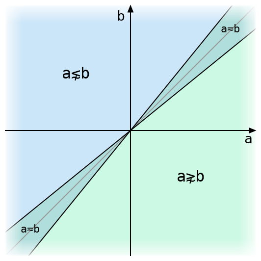
The above figure illustrates tolerant comparison of two real numbers. They are exactly equal only on the grey diagonal line, and tolerantly equal within the narrow strip around it. The diagram uses a much larger value for ⎕CT than Dyalog’s default of 1e¯14, or even its maximum allowed value of 2*¯32, either of which would make that strip invisible.

One way to define tolerant inequalities in terms of tolerant equality is to define, for instance, (a≲b) ≡ (a<b)∨(a≂b) using intolerant less-than and tolerant equality. But we’ll find it more useful to define and directly in terms of intolerant comparisons as with . The formula for is:

(a-b) ≤ ⎕CT × 0⌈a⌈-b

and for we can use either (a≳b) ≡ (b≲a) or (a≳b) ≡ (-a)≲(-b) to obtain

(b-a) ≤ ⎕CT × 0⌈b⌈-a

or, negating both sides and swapping the inequality,

(a-b) ≥ ⎕CT × 0⌊a⌊-b

The 0⌈ term isn’t strictly necessary (as we’ll show later), but it helps avoid some confusion when a and b have different signs. Sometimes it’s used to speed up comparison by checking if a≤b intolerantly before performing any multiplication—if it is, the multiplication isn’t needed.

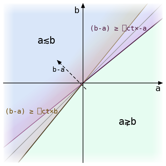
Above we can see how the equation for tolerant splits into two symmetrical half-formulas, each of which is just a little off from the exact inequality a≤b. The tolerant inequality accepts either of these conditions.

The region of tolerant equality is now the intersection of the regions for tolerant and . That is:

(a≂b) ≡ (a≲b)∧(a≳b)

We’ll find this decomposition handy later on since tolerant inequalities are so much easier to work with.

Tolerating an inequality

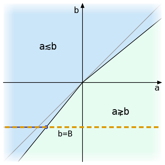
What happens if we fix one side of the inequality? Here’s a diagram for a≲b with a dashed line drawn where b is equal to some fixed B and a varies.

There’s only one place where the black line bounding the region where a≲b intersects the line b=B. The value of a at this intersection has an interesting property: when a is (exactly) less than or equal to that value, then it is tolerantly less than or equal to B. If we want to compare B to many other floating-point values, and we know the a coordinate of the intersection above, then we can skip all of the tolerant comparison arithmetic and just use exact comparison with that value!

Once we have a way to do this for all other inequalities will follow, since (a≳B) ≡ (-a)≲(-B) and (a⋧B) ≡ ~(a≲B).

Maybe you can figure out the value from the graphs above. But it’s also easy to find the value (and prove it works!) using a fact about the maximum function: for real numbers x, y, and z, x≤y⌈z is the same as (x≤y) ∨ (x≤z). One of the advantages of treating inequalities as functions like any other is that formulas like these are easy to manipulate. Here we go:

Start with the formula for tolerant inequality, writing q in place of ⎕CT.

(a-B) ≤ q × 0⌈a⌈-B

Distributing over , we have

(a-B) ≤ 0 ⌈ (q×a) ⌈ (-q×B)

and using (x≤y⌈z) ≡ ((x≤y) ∨ (x≤z)) twice (just like in the previous step, this can be thought of as distributing x≤ over three arguments of an associative function all at once), we can expand this formula to

((a-B) ≤ 0) ∨ ((a-B) ≤ q×a) ∨ ((a-B) ≤ -q×B)

which simplifies to

(a ≤ B) ∨ ((a×1-q) ≤ B) ∨ (a ≤ B×1-q)

or (here we need q<1, so that 1-q is positive; otherwise we’d have to reverse the middle inequality)

(a ≤ B) ∨ (a ≤ B÷1-q) ∨ (a ≤ B×1-q)

Recombining, we get

a  ≤  B ⌈ (B÷1-q) ⌈ (B×1-q)

So that’s our formula: now the tolerant equality is an intolerant equality, where the right side depends only on B!

Reading the signs

So we have a formula for a “tolerated” value b = B ⌈ (B÷1-q) ⌈ (B×1-q). When do the different possible maxima come into play?

  • If B=0, then everything on the right is zero, and b=0.
  • If B>0, then B×1-q is smaller than B, since q>0. But that means ÷1-q is larger than 1, and B÷1-q is larger than B. So b=B÷1-q.
  • If B<0, then the all the inequalities that we got with B>0 are reversed. This means b=B×1-q.

Note that none of these cases depend on the branch b=B, even though the first one touches it. That means the definition of tolerant inequality would be the same even if we remove that branch. By working backwards through the above derivation we find that the initial 0⌈ has no effect, and we can remove it from the definition.

Equality

Tolerant equality obviously can’t be reduced to intolerant equality, since many values can be tolerantly equal to a number but only one is intolerantly equal to it. But recalling that (a≂b) ≡ (a≲b)∧(a≳b), we can express it as two intolerant inequalities: tolerate b for as above. Then tolerate it for (this always yields a value at least as large as the first). a is tolerantly equal to b if it lies between the two tolerated values.

This case is particularly important for the set functions ⍳∊∩∪~, which by definition use tolerant equality to match values in one argument to values in the other. If the non-principal argument (the one containing values to be looked up, like the right argument to ) is short enough, then each element in it is looked up using a simple linear search through the principal argument. This means that one number at a time is compared to the entire principal argument (up to the first match found). So for floats we can get a substantial improvement by tolerating each element on the right before comparison.

Caution!

That was the easy part.

In this post we’ve been assuming that floating-point numbers behave like mathematical real numbers. Given that the whole reason tolerant comparison was introduced is that they don’t, maybe that wasn’t the best assumption.

The formulas B÷1-q and B×1-q for tolerated comparison are flawed: they produce values that differ slightly from the actual number that should be used in an intolerant equivalent to tolerant comparison. This is very dangerous: many programs could break if two values compare equal in one comparison but not in another! In the next post we’ll dive into the world of floating-point error analysis and find out how to get the right values. And we’ll discover that imperfect computation isn’t all bad when we find a faster alternative to a very slow floating-point division.