Turning to a Heading with an MPU-9150

Posted on September 8, 2014 by Morten Kromberg

As the odour of fried electronics dissipates in the air, I’m unexpectedly afforded the opportunity to write this blog post a day or two earlier than planned. The on-board compass was exhibiting significant deviation, so I consulted my nephew Thorbjørn Christensen at DTU-Space. Thorbjørn makes a living designing magnetometers for space agencies around the world, and he suggested I use a ribbon cable to move the IMU away from the bot as a first step towards understanding the issue. He did warn me to be very careful when attaching it. I still don’t understand what I did wrong, but the evidence that I screwed up is pretty definitive: there are burn marks around every single connector and the IMU chip looks a bit soft in the middle. Most importantly, it no longer reports for duty on the Raspberry Pi’s I2C bus!

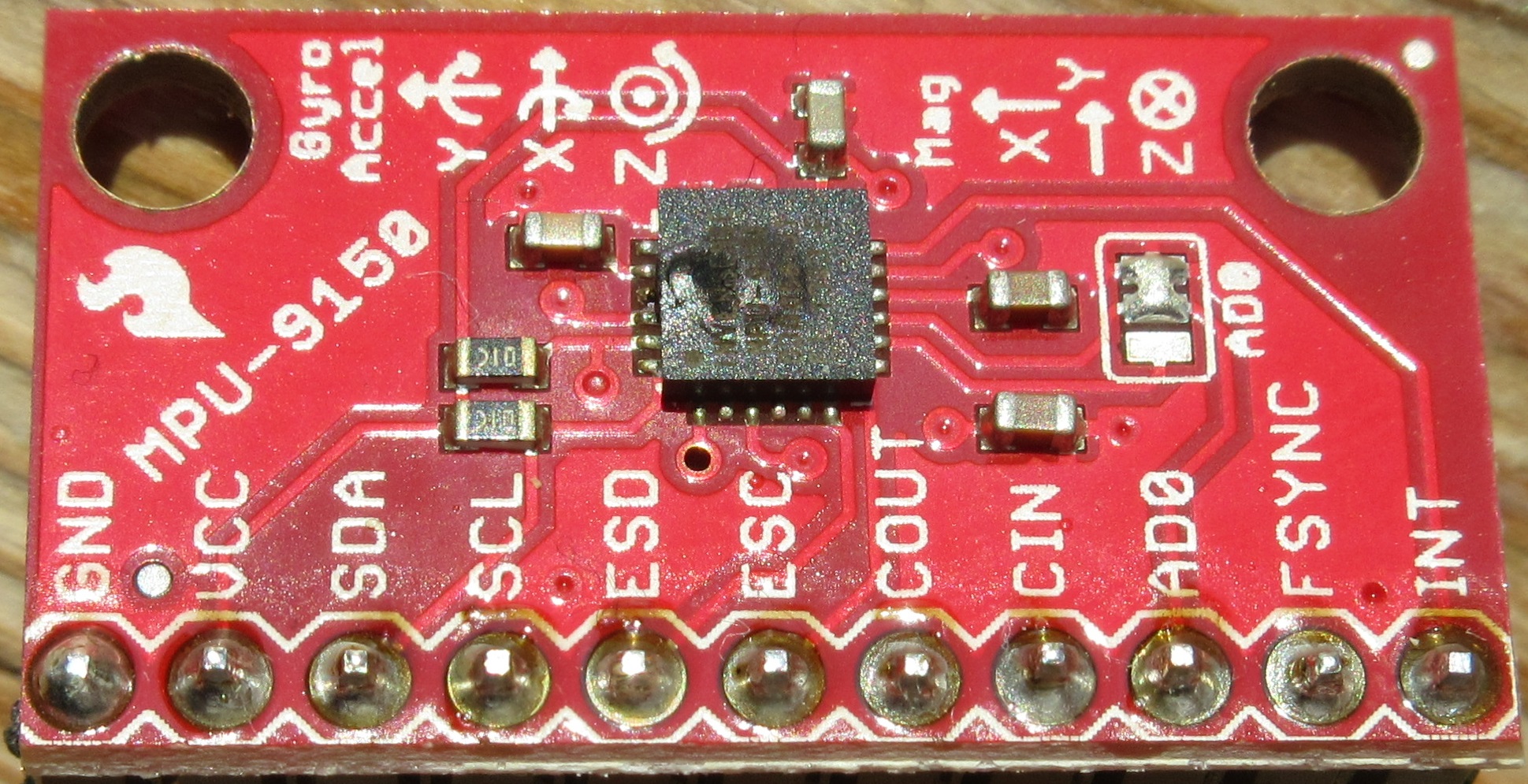
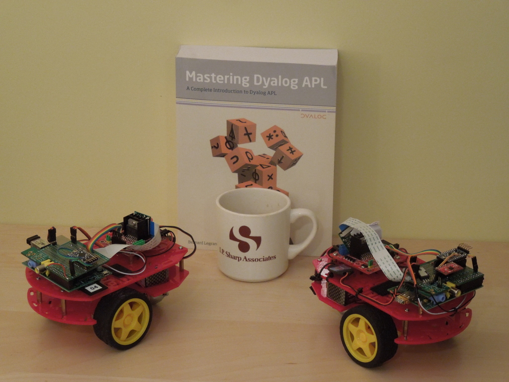
A fried IMU-9150 (click to enlarge)

The good news (apart from the fact that the Raspberry Pi, the Arduino and all other ‘bot components seem to have survived) is perhaps that, since I cannot play with the compass until I have a replacement, I found the time to write about where I am at the moment…and take some time out to work on my presentations for Dyalog ’14 (for those who managed to register before the user meeting in Eastbourne sold out, I still hope to do a ‘bot presentation on the evening of Tuesday September 23rd).

Introducing the MPU-9150

For the last few weeks, I have been using my “bot time” to play with the MPU-9150 breakout board that is attached to our ‘bot. The MPU-9150 is more or less identical to the 6050 that we were using earlier this summer to make gyro-controlled turns but also includes a magnetic compass, which will allow us to know the direction that we are heading in – making it a 9 degree of freedom inertial measurement unit, or “9-dof IMU” (9 = 3 gyro axes + 3 accelerometer axes + 3 compass axes).

RTIMULib

I was extremely happy to discover that Richard Barnett had shared his RTIMULib on GitHub. RTIMULib is a Linux library that produces “Kalman-filtered quaternion or Euler angle pose data” based on data from a 9-dof IMU. Jay Foad at Dyalog was quickly able to provide me with a couple of additional C functions designed to be easy to call from Dyalog APL. Jay’s fork of RTIMULib is also available on GitHub. Since we can assume that we are driving on a flat surface, I have just been using two items from the wealth of information provided by this library: the current rate of rotation and the current compass direction – in both cases around the vertical (or “z”) axis.

My First Compass-Controlled Rotation

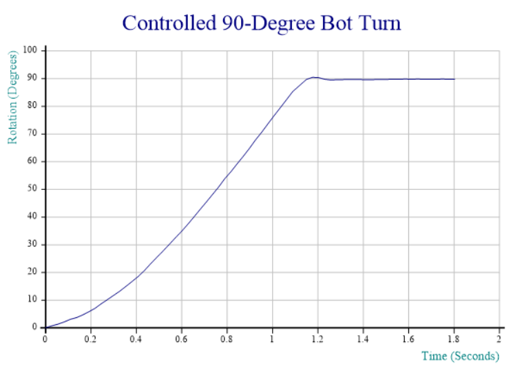
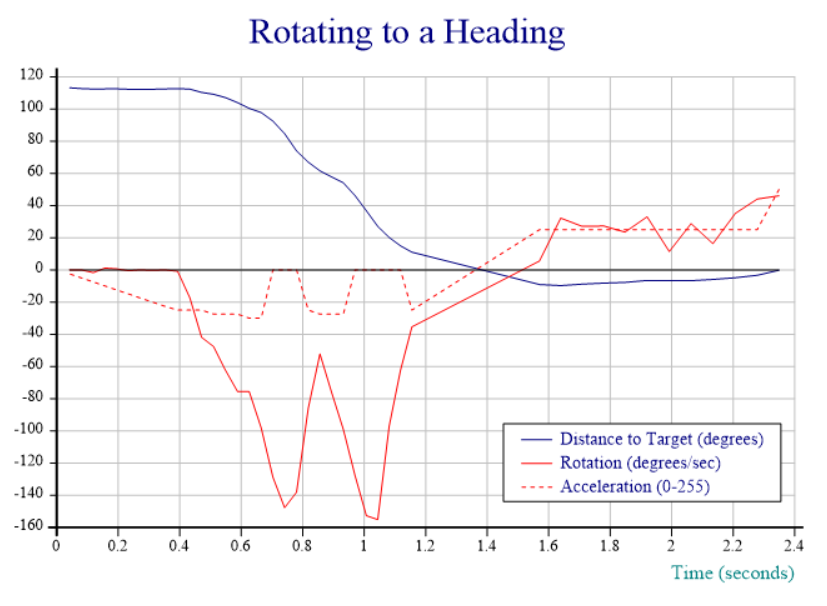
Due to the fried IMU, I am unable to post a video recording; fortunately, at the moment where I toasted the chip, the Dyalog session output still contained output data from the last run of the function I am working on, which aims to provide smooth rotation to a selected compass heading. In the chart below, the red line tracks the speed of rotation and shows that the “smooth” part still needs work – the speed oscillates quite violently between 60 and 150 degrees per second. The blue line shows the number of degrees that the ‘bot still needs to turn to reach the desired heading. The dotted red line is slightly mislabeled: rather than acceleration, it actually shows the power applied to the motors via a digital-to-analog converter that accepts values between 0 and 255, producing between 0 and 5v of voltage for the DC motors:

Commentary:

From 0 to 0.4 seconds, we slowly increase power until we detect that rotation has started. We note the power setting required to start rotation.
0.4 to 0.7 (ish), we detect acceleration and hold the throttle steady (increasing it very slightly a couple of times when acceleration appears to stop).
0.7 to 1.1 seconds, cruise mode: whenever speed is above the target of 100 degrees/sec, we idle. When speed is below 100, we re-apply power at a level that was sufficient to start the rotation.
1.1 to 1.4 seconds: We are less than 30 degrees from target, and the target velocity and thus power is reduced proportional to the remaining distance (at 15 degrees, we are down to 50 deg/sec)
1.4 to 1.6 seconds: We detect that we rotated too far, and slam on the brakes, coming to a stop about 10 degrees from target.
1.6 to 2.3 seconds: since we are less than 10 degrees from target, we enter “step” mode, giving very brief bursts of power at “start rotation” level, idling, and watching the heading until we reach the goal.
2.4 seconds: We count the bursts and, after 10, we double the power setting to avoid getting bogged down (you cannot see the bursts in the chart, it only records the power level used for each one). A little more patience would have been good, this probably means we overshot by a bit.

The “Heading” Function

Achieving anything resembling smooth movement is still some way away, mostly due to the fact that motor response to a given input voltage varies enormously from motor to motor and between different applications to the same motor. The strategy described above is implemented by a function named “Heading”, which can be found in the file mpu9150.dyalog in the APLBot folder on GitHub. An obvious improvement would be to have the robot self-calibrate itself somehow and add a model of how fast rotation speeds up and slows down (based on, and constantly adjusted with, observed data), in order to dampen the oscillations. I intend to return to this when I have a new IMU (and my other user meeting presentations are under control).

This has turned out to be a lot harder than I imagined: suggestions are very welcome – please leave comments if you have a good idea!

Making Controlled Turns with the DyaBot

Posted on August 11, 2014 by Morten Kromberg

This blog originally started when I took delivery of the DyaBot, a Raspberry Pi and Arduino based variant of the C3Pi running Dyalog v13.2. The architecture of the ‘bot and instructions for building your own inexpensive robot can all be found in blog entries from April to July of last year.

The downside of only using inexpensive components is that some of them are not very precise. The worst problem we face is that the amount of wheel movement generated by the application of a particular power level varies from one motor to the next, and indeed from moment to moment. Trying to drive a specific distance in a straight line, or make an exact 90 degree turn regardless of the surface that the ‘bot is standing on, are impossible tasks with the original Dyabot. You can have a lot of fun, as I hope the early posts demonstrate, but we have higher ambitions!

Our next task is to add motion sensors to the DyaBot, with a goal of being able to measure actual motion with sufficient accuracy to maintain our heading while driving straight ahead – and to make exact turns to new headings, like the 90-degree turn made in this video (the ‘bot has been placed on a Persian carpet to provide a background containing right angles):

Introducing the MPU-6050

For some time we have had an MPU-6050, which has 3-axis rotation and acceleration sensors, attached to our I2C bus, but haven’t been able to use it. About ten days ago (sorry, I took a few days off last week), @RomillyC came to visit us in Bramley to help me read some Python code that was written for this device. The current acceleration or rotation on each axis is constantly available as a register and can be queried via I2C. Translated into APL, the code to read the current rate of rotation around the vertical axis is:

 ∇ r←z_gyro_reading ⍝ current z-axis rotation in degrees
   r←(read_word_2c 70)÷131 ⍝ Read register #70 and scale to deg/sec
 ∇

 ∇ r←read_word_2c n;zz
   r←I2 256⊥read_byte_2c¨n+0 1               ⍝ Read 2 registers and make signed I2
 ∇

 ∇ r←read_byte_2c n;z
   z←#.I2C.WriteArray i2c_address (1,n)0     ⍝ Write register address
   r←2 2⊃#.I2C.ReadArray i2c_address (1 0)1  ⍝ Read input
 ∇

 I2←{⍵>32767:1-65535-⍵ ⋄ ⍵} ⍝ 16-bit 2's complement to signed

Integrating to Track Attitude

Reading the register directly gives us the instantaneous rate of rotation. If we want to track the attitude, we need to integrate the rates over time. The next layer of functions allows us to reset the attitude and perform very primitive integration by multiplying the current rotation with the elapsed time since the last measurement:

∇ r←z_gyro_reset            ⍝ Reset Gyro Integration
  z_gyro_time←now           ⍝ current time in ms
  z_gyro_posn←0             ⍝ current rotation is 0
∇

∇ r←z_gyro;t;delta          ⍝ Integrated gyro rotation
  t←now                     ⍝ current time in ms
  delta←0.001×t-z_gyro_time ⍝ elapsed time in seconds
  r←z_gyro_posn←z_gyro_posn+delta×z_gyro_reading+z_gyro_offset
  z_gyro_time←t             ⍝ last time
∇

We can now write a function to rotate through a given number of degrees (assuming that the gyro has just been reset): we set the wheels in motion, monitor the integrated angle until we are nearly there, then shut off the engines. We continue logging the angles for a brief moment to monitor the deceleration. The function returns a two-column matrix containing the “log” of rotation angles and timestamps:

    ∇ log←rotate angle;bot;i;t
     
      log←0 2⍴0 ⍝ Angle, time
      bot.Speed←3 ¯3 ⍝ Slow counter-clockwise rotation
     
      :Trap 1000 ⍝ Catch interrupts
          :Repeat
              log⍪←(t←z_gyro),now
          :Until t>angle-7 ⍝ Stop rotating 7 degrees before we are done    
      :EndTrap

      bot.Speed←0 ⍝ cut power to the motors
      :For i :In ⍳25 ⍝ Capture data as we slow down
          log⍪←z_gyro,now
      :EndFor
    ∇

The logged data from the rotation captured in the video at the top is charted below:

Even with the primitive integration and rotation strategies, the results already look quite promising. I’ll be taking most of this week off – part of it without access to the internet(!), but once I am back, expect the next blog entry to explore writing functions that accelerate and slow down in a more controlled fashion as well as stop at the right spot rather than relying on a specific amount of friction to rotate through the last 7 degrees (note the very slight reverse rotation at the end, probably caused by the Persian carpet being a bit “springy”). I will also clean up the code and post the complete solution on GitHub – and perhaps even look at some better integration techniques.

If you would like to make sure you don’t miss the next installment, follow the RSS feed or Dyalog on Twitter.

Dancing with the Bots

Posted on August 2, 2014 by Morten Kromberg

Last week the ‘bots were busy preparing for the J Language Conference in Toronto, where they made their first public appearance together. Upon returning to Bramley they continued training and we are proud to present the first recording of their new dance:

The ‘bots are both running the same DyaBot class as last year. This class exposes a property called Speed, which is a 2-element vector representing the speed of the right and left wheels respectively. Valid values range from +100 (full speed ahead) to -100 (full reverse). The annotations displayed at the top left show the settings used for each step of the dance.

Controlling Two Robots at Once using Isolates

Isolates are a new feature included with Dyalog version 14.0, designed to make it easy to perform distributed processing. In addition to making it easy to used all the cores on your own laptop or workstation, isolates make it possible to harness the power of other machines. This requires the launching of an “isolate server” on each machine that wants to offer its services:

Starting an isolate server using PuTTY to run Dyalog on the robot.

Starting an isolate server on DyaBot00 using PuTTY.

Once we have an isolate server running on each robot we can take control of them from a remote session as follows:

      )load isolate
      #.isolate.AddServer 'dyabot00' (7052)      
      #.isolate.AddServer 'dyabot04' (7052)
      bots←isolate.New¨Bot Bot
      bots.Init
 dyabot00  dyabot04

Above, we create two instances of the Bot namespace. The expression Bots.Init invokes the Init function, which returns the hostname, in each isolate:

:Namespace Bot

    ∇ r←Init;pwd
      pwd←∊⎕SH'pwd' ⍝ Find out where to copy from
      #.⎕CY botws←pwd,'/DyaBot/DyaBot.dws' ⍝ copy ws
      i←⎕NEW #.DyaBot ⍬ ⍝ Make DyaBot instance    
      r←⎕SH'hostname' ⍝ Return hostname
    ∇

:EndNamespace

Next, we define a function “run” that will take a vector of dance steps as input. Each step is a character vector (because that makes editing slightly easier!) containing five numbers: The first two set the speed of one robot, the next two the speed of the other and the fifth defines the duration of the step. After each step we pause for a second, to give humans time to appreciate the spectacle:


    ∇ run cmds;data;i;cmd;z
[1]    ⎕DL 5
[2]    :For i :In ⍳≢cmds
[3]        :If ' '∨.≠cmd←i⊃cmds
[4]            data←1 0 1 0 1⊂2⊃⎕VFI cmd ⍝ Cut into 3 numeric pieces
[5]            z←bots.{i.Speed←⍵}2↑data ⋄ ⎕DL⊃¯1↑data ⋄ z←bots.(i.Speed←0)
[6]            ⎕DL 1
[7]        :EndIf
[8]    :EndFor
    ∇

Now we are ready to roll: Call the run function with a suitable array and watch the robots dance (see the video at the top)!

      ↑choreography
50  50  0   0 1.5
 0   0 50  60 1.2
50 ¯50 50 ¯50 0.3
20  80 10  70 5  
50 ¯50 50 ¯50 0.3
50  50  0   0 1.5
 0   0 50  60 1.2

      dance choreography

Join us again next week to hear what happened when Romilly came to Bramley to help wire up the accelerometer and gyro!

The Blog is Back!

Posted on July 21, 2014 by Morten Kromberg

It is now 3 weeks since we shipped Dyalog version 14.0 and released the new Dyalog web site, so it’s probably time to stop celebrating and get back to work. The ‘bot batteries have been recharged and the ‘bots are learning to work as a team using v14.0 futures and isolates. That’s all I can say at this time as the ‘bots are rehearsing for a gig at the J Conference on Friday 25th July and I have been sworn to secrecy until after the show.

Bots 00 and 04 preparing for the J Conference and thinking about whether to attend the IPSA 50th renunion on October 4th

Bot 04 and Bot 00 hanging out in Rochester NY rehearsing for the J Conference and considering whether to return to Toronto with me for the IPSA 50th reunion on October 4th this year.

The next major step in the robot project is to make use of the tiny red board attached to Bot 00 (on the right) – an MPU-6050 accelerometer. At the Dyalog Seminar in New York last Thursday I finally had the pleasure of meeting @alexcweiner in person, and we vowed to crack this nut together; since @romillyc has promised to join in as well, failure is not an option. Stay tuned to hear more about that adventure in the weeks to come!

Welcome to The Development Team Blog

The really good news is that this blog is no longer simply “the CTO blog” but a blog that will be shared by the entire development team as well as invited guests. We look forward to sharing details of the things we are working on with you all…

APL-Controlled Robot Performs Death-Defying Stunts Using PiCam

Posted on September 2, 2013 by Morten Kromberg

Regular readers will remember my whining about the poor precision of both infra-red and ultrasonic sensors. But today, the Raspberry Pi / Dyalog APL – controlled “DyaBot” was observed driving on a dinner table – where the slightest navigational error could mean a 3-foot plunge and certain death! How can this be?

The answer is: the “PiCam” finally arrived last week!!!

Capturing Images with The PiCam

I no longer need to complain about sonar beams being up to 30 degrees wide: the PiCam has a resolution of up to 1080×1920 pixels! So all we need is some software to interpret the bits…First, we capture images using the “raspistill” command:

raspistill -rot 90 -h 60 -w 80 -t 0 -e bmp -o ahead.bmp

The parameters rotate the image 90 degrees (the camera is mounted “sideways”), set the size to 60 x 80 pixels (don’t need more for navigation), take the picture immediately, and store the output in a file called “ahead.bmp”. (Documentation for the camera and related commands can be found on the Raspberry Pi web page.) Despite the small number of pixels, the command takes a full second to execute – anyone who knows a way to speed up the process of taking a picture, please let me know!

In the video, each move takes about 3 seconds, this is simply because each cycle is triggered by a browser refresh of the page after 3 seconds. Capturing the image takes about 1 second, the “image analysis” about 40 milliseconds, so we could be driving a lot faster with a bit of Javascript on the client side (watch this space).

Extracting BitMap Data

Under Windows, Dyalog APL has a built-in object for reading BitMap files, but at the moment, the Linux version does not have an equivalent. Fortunately, extracting the data using APL is not very hard (after you finish reading about BMP files on WikiPedia):

tn←'ahead.bmp' ⎕NTIE 0     ⍝ Open "native" file
(offset hdrsize width height)←⎕NREAD tn 323 4 10 
                           ⍝ ↑↑↑ Read 4 Int32s from offset 10
data←⎕NREAD tn 80 (width×height×3) offset ⍝ Read chars (type 80)
data←⊖⎕UCS(height width 3)⍴data ⍝ Numeric matrix, reverse rows

The above gives us a 60 by 80 by 3 matrix containing (R,G,B) triplets. This code assumes that BMP file is in the 24-bit format created by raspistill; I will extend the code to handle all BMP formats (2, 16 and 256 colours) and post it when complete – but the above will do for now.

Where’s the Edge?

At Iverson College last week, I demonstrated the DyaBot driving on a table with a green tablecloth, using code which compared the ratio between R,G,B values to an average of a sample of green pixels from one shot. Alas, I prepared the demo in the morning and, when the audience arrived, there was much more (yellowish) light coming in through the window. This changed the apparent colour so much that the bot decided that the side of the table facing the window was now unsafe, and it cowered in the darkness.

Fortunately, I was talking to a room full of very serious hackers, who sent me off to Wikipedia to learn about “kernels” as a tool for image processing. Armed with a suitable edge detection kernel, I was able to test this new algorithm on a dozen shots taken at different angles with the PiCam. Each pair of images below has the original on the left, and edges coloured red on the right. Notice that, although the colour of the table varies a lot when viewed from different directions – especially when there is background glare – the edges are always correctly identified:

Except for the image at the bottom left, where the bot is so close to the edge that the table is not visible at all (and the edge is the opposite wall of the room, ten feet away), we seem to have a reliable tool.

The PiServer Page

The code to drive the bot is embedded in a “PiServer” (MiServer running on a Rasperry Pi) web page. Each refresh of the page takes a new picture, extracts the bits, and calls the main decision-making function. The suggested action (turn or drive straight ahead) is displayed in the form, and the user has the choice of pressing OK to execute the command, pressing the “Nah” button to take a new photo and try again (after moving the bot, changing the lighting in the room, or editing the code). There are also four “manual” buttons for moving the Bot. After testing the decision-making abilities of the code, brave programmers press the “Auto” button, allowing the robot to drive itself without waiting for confirmation before each command (see the video at the start of this post)!

The Code

The central decision-making function and the kernel computation function are listed below. The full code will be uploaded to the MiServer repository on GitHub, once it is finally adjusted after I find a way to attach the PiCam properly, rather than sticking it to the front of the Bot with a band-aid!

∇ r←StayOnTable rgb;rows;cols;table;sectors;good;size;edges
 ⍝ Based on input from PiCam, drive at random, staying on table
 ⍝ Return vector containing degrees to turn and 
 ⍝               #seconds to drive before next analysis

 (rows cols)←size←2↑⍴rgb
 ⍝ First detect edges in each colour separately
 edges←EdgeDetectAll∘AK¨⊂[1 2]rgb
 ⍝ Call it an edge if any r, g or b result is >75% of original
 edges←∨/(↑[0.5]edges)>0.75×1 1↓¯1 ¯1↓rgb
 ⍝ Look for lowest edge in each column 
 table←+⌿∧⍀~⊖edges
 ⍝ Divide into 3 equally sized sectors (left, centre, right) 
 sectors←((⍴table)⍴(⌈(⍴table)÷3)↑1)⊂table
 ⍝ Find the LOWEST edge in each sector
 good←⌊/¨sectors

 :If good∧.>15 ⍝ More than 15 pixel rows of table in all sectors
    r←0,0.1⌈(good[2]-15)÷25 ⍝ Carry straight on for a while
 :Else ⍝ Some sectors have less than 15 pixel rows
    :If 0≠1↑previous ⋄ r←previous 
        ⍝ Once started turning, keep turning the same way
    :Else 
        r←((1+>/good[1 3])⊃45 ¯45),0 ⍝ Turn in "best" direction
    :EndIf
 :EndIf
 previous←r ⍝ Remember last turn for next decision
∇

The function AK (Apply Kernel), and the kernel are defined as follows:

∇ r←kernel AK data;shape
   shape←⍴kernel
   r←(1-shape)↓⊃+/,kernel×(¯1+⍳1↑shape)∘.⊖(¯1+⍳1↓shape)∘.⌽⊂data
∇

 EdgeDetectAll ⍝ Our 3x3 kernel
¯1 ¯1 ¯1
¯1  8 ¯1
¯1 ¯1 ¯1

Note the similarity of AK to the APL Code for Conway’s Game of Life!

Comparing Sonar and InfraRed Data

Posted on August 16, 2013 by Morten Kromberg

Of course, it was an illusion that I would be able to get straight back to the robot after vacation, there were a few other jobs waiting like the Dyalog’13 Conference Programme (the DyaBot will be making a couple of appearances, of course!). However, it appears I have now made enough flour to be able to remove my nose from the grindstone for a bit and spend more time with the robot, so I expect to be back to posting every week or so from now on, as we prepare to demonstrate an autonomously navigating robot at the conference!

Anyhow, here is a chart with the first recorded data from the LV-EZ4 ultrasonic sensor (sonar) – using RainPro, as demonstrated in the post on visualising sensor data. Many thanks to Stefano Lanzavecchia for help with the math required to generate the co-ordinates of a rectangle in a polar chart:

The robot was placed in my kitchen (the setting for several robot videos), about 80cm from the back wall, 240cm from the front, and roughly halfway between the sides. The green rectangle labelled “actual” above shows the location of the walls relative to the bot. It was commanded to rotate through 360 degrees, recording the readings from the IR (red line) and Sonar (blue) sensors, which were both pointing straight ahead. Ideally, the blue line should have traced an identical rectangle. The red line essentially traces an 80cm circle plus noise, this is because SHARP GP2Y0A21YK0F infrared sensor has a maximum range of 80cm.

Sonar Issues

The ultrasonic sensor has a range of at least 6-7m, and is our choice for long-range distance measurements. However, what I believe the graph shows, is that we have a serious problem with reflections. Essentially, it appears that when the sonar beam hits a wall at certain angles, there is very little direct return; instead the beam is reflected. The return signals that we are getting from roughly 60 and 315 degrees look like reflections of the back wall – these reflections may be enhanced by the fact that there is a refrigerator at 60 and a dishwasher at 315 (metal surfaces). The signals at 135 and 220 degrees could be reflections of the robot itself, the beam having been reflected twice in a corner of the room.

Another thing that is not immediately evident from the above image, but took me by surprise studying the data sheet, was that the sonar beam is a quite a bit wider than I expected – as much as 30 degrees at close range, getting narrower as the distance increases (see the data sheet). In other words, we have some work to do in order to generate accurate maps of the universe based on the current set of sensors.

Will we succeed? To be continued …

The tool of thought for

software solutions

Contact Us

Category Archives: Robots