Diane’s Lasagne Problem

Making Lasagne

Participants in the SA2 Performance Tuning workshop at the Dyalog ’18 User Meeting were encouraged to bring their own problems for the group to work on. Diane Hymas of ExxonMobil brought a good one. The one-liner computation is as follows:

lasagne0 ← {groups {+⌿⍵}⌸ amts ×[⎕io] spices[inds;]}

where

   n ← 8e5
   spices ← ?6000 44⍴0
   groups ← +\(16↑1 2)[?n⍴16]
   inds   ← ?n⍴≢spices
   amts   ← ?n⍴0

Applying lasagne0 to this dataset:

   ⍴ lasagne0 ⍬
100015 44
   ≢ ∪ groups
100015

   )copy dfns wsreq cmpx

   wsreq 'lasagne0 ⍬'
844799820
   cmpx  'lasagne0 ⍬'
2.12E¯1

The problem with lasagne0 is space rather than time. The 845 MB required for this dataset may be acceptable, but we can be called upon to cook up large batches of lasagne in a smallish workspace, on a machine with limited RAM. (Large n and large ≢∪groups.)

All benchmarks in this document were run in Dyalog APL version 17.0, in a 2 GB workspace, on a machine with generous RAM.

Solutions

Marshall Lochbaum solved the problem. The alternative solutions are as follows:

lasagne0 ← {groups {+⌿⍵}⌸ amts ×[⎕io] spices[inds;]}
lasagne1 ← {↑ (groups{⊂⍵}⌸amts) {+⌿⍺×[⎕io]spices[⍵;]}¨ groups{⊂⍵}⌸inds}
lasagne2 ← {↑ (groups{⊂⍵}⌸amts)      {⍺+.×spices[⍵;]}¨ groups{⊂⍵}⌸inds}
lasagne3 ← {↑ {amts[⍵]+.×spices[inds[⍵];]}¨ {⊂⍵}⌸groups}

lasagne0 is the original expression; lasagne1 and lasagne2 were derived by Marshall during the workshop; lasagne3 was suggested by a participant in the workshop. The four functions produce matching results. Comparing the space and time:

space (MB)           time
lasagne0 845 2.29e¯1 ⎕⎕⎕⎕⎕⎕⎕⎕⎕⎕⎕⎕⎕⎕⎕⎕⎕⎕⎕
lasagne1 74 3.60e¯1 ⎕⎕⎕⎕⎕⎕⎕⎕⎕⎕⎕⎕⎕⎕⎕⎕⎕⎕⎕⎕⎕⎕⎕⎕⎕⎕⎕⎕⎕⎕
lasagne2 74 2.39e¯1 ⎕⎕⎕⎕⎕⎕⎕⎕⎕⎕⎕⎕⎕⎕⎕⎕⎕⎕⎕⎕
lasagne3 74 2.93e¯1 ⎕⎕⎕⎕⎕⎕⎕⎕⎕⎕⎕⎕⎕⎕⎕⎕⎕⎕⎕⎕⎕⎕⎕⎕

lasagne0 v  lasagne1

Nearly all of the space required to evaluate lasagne0 is accounted for by the space for computing the right argument to key:

   wsreq 'lasagne0 ⍬'
844799820

   wsreq 'amts ×[⎕io] spices[inds;]'
844799548

In fact, the array spices[inds;], all by itself, is already very large. It has shape (⍴inds),1↓⍴spices (≡ 8e5 44), each item requiring 8 bytes.

   wsreq 'spices[inds;]'
281599556

   ⍴ spices[inds;]
800000 44

   8 × ×/ ⍴ spices[inds;]
281600000

   qsize←{⎕size '⍵'}    ⍝ # bytes for array ⍵
   qsize spices[inds;]
281600040

lasagne1 avoids creating these large intermediate results, by first partitioning the arguments (groups{⊂⍵}⌸amts and groups{⊂⍵}⌸inds) and then applying a computation to each partition. In that computation, the operand function {+⌿⍺×[⎕io]spices[⍵;]}, is a partition of amts and is the corresponding partition of inds.

lasagne1, lasagne2 and lasagne3 require the same amount of space to run, so the comparison among them is on time.

lasagne1 v  lasagne2

The only change is from +⌿⍺×[⎕io]spices[⍵;] to ⍺+.×spices[⍵;], which are equivalent when is a vector. The interpreter can compute +.× in one go rather than doing +⌿ separately after doing ×[⎕io]; in such computation the interpreter can and does exploit the additional information afforded by +.× and is faster by a factor of 1.5 (= 2.39 ÷⍨ 3.60).

lasagne2 v  lasagne3

The idea in lasagne3 is doing one key operation rather than the two in lasagne2. Therefore, the changes between lasagne2 v lasagne3 are:

lasagne2 groups{⊂⍵}⌸amts
groups{⊂⍵}⌸inds
spices[⍵;]
lasagne3 {⊂⍵}⌸groups amts[⍵] spices[inds[⍵];]

All three key operations involve {⊂⍵}⌸ with groups as the key, and are roughly equally fast, each taking up no more than 7% of the total time.

   cmpx 'groups{⊂⍵}⌸amts' 'groups{⊂⍵}⌸inds' '{⊂⍵}⌸groups'
  groups{⊂⍵}⌸amts → 1.69E¯2 |   0% ⎕⎕⎕⎕⎕⎕⎕⎕⎕⎕⎕⎕⎕⎕⎕⎕⎕⎕⎕⎕⎕⎕⎕⎕⎕⎕⎕⎕⎕⎕
* groups{⊂⍵}⌸inds → 1.39E¯2 | -18% ⎕⎕⎕⎕⎕⎕⎕⎕⎕⎕⎕⎕⎕⎕⎕⎕⎕⎕⎕⎕⎕⎕⎕⎕⎕
* {⊂⍵}⌸groups     → 1.36E¯2 | -20% ⎕⎕⎕⎕⎕⎕⎕⎕⎕⎕⎕⎕⎕⎕⎕⎕⎕⎕⎕⎕⎕⎕⎕⎕

lasagne3 is doing one less key operation than lasagne2 in exchange for doing, for each of the ≢∪groups (= 100015) executions of the operand function, amt[⍵] v and spices[ind[⍵];] v spices[⍵;]. Indexing is by no means slow, but it’s not as fast as references to and . Therefore, lasagne2 is faster.

The trade-off may differ for different values of groups. In this case groups are small-range integers so operations using it as the key value are fast.

Permuting Internal Letters

Friday Afternoon

It’s something of a custom in Dyalog to send a “fun” e-mail to the group on Friday afternoons. My gambit for this past Friday was:

   x ←' according to research it doesn''t matter'
   x,←' what order the letters in a word are'
   x,←' the human mind can still read it'
   x,←' the only important thing is that'
   x,←' the first and the last letters are in the right place'

   ∊ ' ',¨ {(1↑⍵),({⍵[?⍨≢⍵]}1↓¯1↓⍵),(-1<≢⍵)↑⍵}¨ (' '∘≠ ⊆ ⊢) x
 aroidnccg to reasrech it dneso't mttear waht order the ltreets 
      in a wrod are the hmaun mnid can sltil read it the olny 
      imartpnot tihng is that the fsrit and the lsat lterets 
      are in the rhigt palce

(The research: http://www.mrc-cbu.cam.ac.uk/people/matt.davis/Cmabrigde/rawlinson/)

Code Golfing

The code golfers were not long in responding:

   ∊{' ',⍵[1,(1+?⍨0⌈¯2+n),n/⍨1<n←≢⍵]}¨(' '∘≠⊆⊢)x     ⍝ fa
   ∊{' ',⍵[∪1,{⍵,⍨?⍨⍵-1}≢⍵]}¨(' '∘≠⊆⊢)x              ⍝ fb
   '\S+'⎕r{{⍵[∪1,{⍵,⍨?⍨⍵-1}≢⍵]}⍵.Match}x             ⍝ fc
   ∊{' ',⍵[n↑1,(1+?⍨0⌈¯2+n),n←≢⍵]}¨(' '∘≠⊆⊢)x        ⍝ fd

In defense of the original expression, it can be said that it follows the pattern:

  • cut into words            (' '∘≠ ⊆ ⊢) x  also ' '(≠⊆⊢)x
  • permute each word      {(1↑⍵),({⍵[?⍨≢⍵]}1↓¯1↓⍵),(-1<≢⍵)↑⍵}¨
  • undo the cut             ∊ ' ',¨

That is, the pattern is “permute under cut”. Moving the ' ', into the permuting function, while shortening the overall expression, obscures this pattern.

Golfing for Speed

One of the code golfers was undaunted by the highfalutin’ functional programming argument. Changing tack, he claimed to be golfing for speed (while himself travelling at 900 kph):

fe←{
  p←1+0,⍸⍵=' '           ⍝ start of each word
  n←0⌈¯3+¯2-/p,2+≢⍵      ⍝ sizes of windows to be shuffled
  ⍵[∊p+?⍨¨n]@((⍳¯1+≢⍵)~p∘.-0 1 2)⊢⍵
}

   cmpx 'fe x' 'fb x' 'fc x' 'fd x'
  fe x → 4.27E¯5 |    0% ⎕⎕⎕⎕
* fb x → 1.05E¯4 | +145% ⎕⎕⎕⎕⎕⎕⎕⎕⎕
* fc x → 3.39E¯4 | +692% ⎕⎕⎕⎕⎕⎕⎕⎕⎕⎕⎕⎕⎕⎕⎕⎕⎕⎕⎕⎕⎕⎕⎕⎕⎕⎕⎕⎕⎕⎕
* fd x → 1.11E¯4 | +159% ⎕⎕⎕⎕⎕⎕⎕⎕⎕⎕

The question was then posed whether the algorithm can be “flattened” further; that is, whether the expression ∊p+?⍨¨n in function fe can be done without each. The answer is of course yes (else I wouldn’t be writing this blog post :-). Flattening, or avoiding the creation of nested arrays, has the potential to reduce memory consumption and increase efficiency, because there is more potential for the interpreter to perform optimized sequential or even parallel operations.

Partitioned Random Permutations

In the old days, before general arrays, before the each and rank operators, ingenious techniques were devised for working with “partitioned” arrays: A boolean vector with a leading 1 specifies a partition on a corresponding array with the same length, basically what we can now do with or similar facility. A detailed description can be found in Bob Smith’s APL79 paper A Programming Technique for Non-Rectangular Data.

   p←1 0 0 1 1 0 0 0 0 0
   v←3 1 4 1 5 9 2 6 53 58

   p⊂v
┌─────┬─┬─────────────┐
│3 1 4│1│5 9 2 6 53 58│
└─────┴─┴─────────────┘

   +/¨ p⊂v
8 1 133
   t-¯1↓0,t←(1⌽p)/+\v
8 1 133

   ∊ +\¨ p⊂v
3 4 8 1 5 14 16 22 75 133
   s-(t-¯1↓0,t←(1⌽p)/⍳⍴p)/¯1↓0,(1⌽p)/s←+\v
3 4 8 1 5 14 16 22 75 133

The last two sets of expressions illustrate how “partitioned plus reduce” and “partitioned plus scan” can be computed, without use of general arrays and without each.

At issue is how to do “partitioned random permute”. Answer: ⍋(n?n)+n×+\p ⊣ n←≢p.

p                1  0  0    1    1  0  0  0  0  0
n?n              5  4 10    6    2  9  8  1  3  7
n×+\p           10 10 10   20   30 30 30 30 30 30
(n?n)+n×+\p     15 14 20   26   32 39 38 31 33 37
⍋(n?n)+n×+\p     2  1  3    4    8  5  9 10  7  6

Therefore:

ff←{
  b←~(⊢ ∨ 1∘⌽ ∨ ¯1∘⌽)' '=⍵  ⍝ internal letters
  n←≢p←b/b>¯1⌽b             ⍝ partition vector for groups of same
  (b/⍵)[⍋(n?n)+n×+\p]@{b}⍵
}

   cmpx 'ff x' 'fe x'
  ff x → 1.46E¯5 |    0% ⎕⎕⎕⎕⎕⎕⎕⎕⎕⎕
* fe x → 4.19E¯5 | +187% ⎕⎕⎕⎕⎕⎕⎕⎕⎕⎕⎕⎕⎕⎕⎕⎕⎕⎕⎕⎕⎕⎕⎕⎕⎕⎕⎕⎕⎕⎕

   x6←1e6⍴x

   cmpx 'ff x6' 'fe x6'
  ff x6 → 5.16E¯2 |    0% ⎕⎕⎕⎕⎕⎕⎕⎕⎕
* fe x6 → 1.77E¯1 | +243% ⎕⎕⎕⎕⎕⎕⎕⎕⎕⎕⎕⎕⎕⎕⎕⎕⎕⎕⎕⎕⎕⎕⎕⎕⎕⎕⎕⎕⎕⎕

There is a puzzle from 1980 which similarly involved randomly permuting items within groups. See A History of APL in 50 Functions, Chapter 47, Pyramigram. The puzzle solution is amusing also for that fact that it used -\.

Afterword

Plobssiy, a txet wshoe words are ilivuddinaly ptemrued is rdeaable mnaliy bseacue in odirrany txet many wrods, eelpclsaiy iptnroamt wrods, are sorht. A curops wtih long and ufnmiailar wdors wuold lkiely be hard to raed atfer scuh pittarmoeun. For eapxmle:

   ff t
 eyonelsmeary dpihnoeissopt siiuqpeedlasan pniormoasaac oopimoentaoa
   ff t
 emlresaneyoy dnpepoihissot seilesiqaadupn poimrnaaasoc oaioomtpneoa
   ff t
 erloymneseay dhsiepopiosnt seildspqiauean praisoaaonmc oomatneiopoa

50847534

⎕io←0 throughout.

I was re-reading A Mathematician’s Apology before recommending it to Suki Tekverk, our summer intern, and came across a statement that the number of primes less than 1e9 is 50847478 (§14, page 23). The function pco from the dfns workspace does computations on primes; ¯1 pco n is the number of primes less than n:

      )copy dfns pco

      ¯1 pco 1e9
50847534

The two numbers 50847478 and 50847534 cannot both be correct. A search of 50847478 on the internet reveals that it is incorrect and that 50847534 is correct. 50847478 is erroneously cited in various textbooks and even has a name, Bertelsen’s number, memorably described by MathWorld as “an erroneous name erroneously given the erroneous value of π(1e9) = 50847478.”

Although several internet sources give 50847534 as the number of primes less than 1e9, they don’t provide a proof. Relying on them would be doing the same thing — arguing from authority — that led other authors astray, even if it is the authority of the mighty internet. Besides, I’d already given Suki, an aspiring mathematician, the standard spiel about the importance of proof.

How do you prove the 50847534 number? One way is to prove correct a program that produces it. Proving pco correct seems daunting — it has 103 lines and two large tables. Therefore, I wrote a function from scratch to compute the number of primes less than , a function written in a way that facilitates proof.

sieve←{
  b←⍵⍴{∧⌿↑(×/⍵)⍴¨~⍵↑¨1}2 3 5
  b[⍳6⌊⍵]←(6⌊⍵)⍴0 0 1 1 0 1
  49≥⍵:b
  p←3↓{⍵/⍳⍴⍵}∇⌈⍵*0.5
  m←1+⌊(⍵-1+p×p)÷2×p
  b ⊣ p {b[⍺×⍺+2×⍳⍵]←0}¨ m
}

      +/ sieve 1e9
50847534

sieve ⍵ produces a boolean vector b with length such that b/⍳⍴b are all the primes less than . It implements the sieve of Eratosthenes: mark as not-prime multiples of each prime less than ⍵*0.5; this latter list of primes obtains by applying the function recursively to ⌈⍵*0.5. Some obvious optimizations are implemented:

  • Multiples of 2 3 5 are marked by initializing b with ⍵⍴{∧⌿↑(×/⍵)⍴¨~⍵↑¨1}2 3 5 rather than with ⍵⍴1.
  • Subsequently, only odd multiples of primes > 5 are marked.
  • Multiples of a prime to be marked start at its square.

Further examples:

      +/∘sieve¨ ⍳10
0 0 0 1 2 2 3 3 4 4

      +/∘sieve¨ 10*⍳10
0 4 25 168 1229 9592 78498 664579 5761455 50847534

There are other functions which are much easier to prove correct, for example, sieve1←{2=+⌿0=(⍳3⌈⍵)∘.|⍳⍵}. However, sieve1 requires O(⍵*2) space and sieve1 1e9 cannot produce a result with current technology. (Hmm, a provably correct program that cannot produce the desired result …)

We can test that sieve is consistent with pco and that pco is self-consistent. pco is a model of the p: primitive function in J. Its cases are:
   pco n   the n-th prime
¯1 pco n   the number of primes less than n
 1 pco n   1 iff n is prime
 2 pco n   the prime factors and exponents of n
 3 pco n   the prime factorization of n
¯4 pco n   the next prime < n
 4 pco n   the next prime > n
10 pco r,s a boolean vector b such that r+b/⍳⍴b are the primes in the half-open interval [r,s).

      ¯1 pco 10*⍳10      ⍝ the number of primes < 1e0 1e1 ... 1e9
0 4 25 168 1229 9592 78498 664579 5761455 50847534

      +/ 10 pco 0 1e9    ⍝ sum of the sieve between 0 and 1e9
50847534
                         ⍝ sum of sums of 10 sieves
                         ⍝ each of size 1e8 from 0 to 1e9
      +/ t← {+/10 pco ⍵+0 1e8}¨ 1e8×⍳10
50847534
                         ⍝ sum of sums of 1000 sieves
                         ⍝ each of size 1e6 from 0 to 1e9
      +/ s← {+/10 pco ⍵+0 1e6}¨ 1e6×⍳1000
50847534

      t ≡ +/ 10 100 ⍴ s
1
                         ⍝ sum of sums of sieves with 1000 randomly
                         ⍝ chosen end-points, from 0 to 1e9
      +/ 2 {+/10 pco ⍺,⍵}/ 0,({⍵[⍋⍵]}1000?1e9),1e9
50847534

      ¯1 pco 1e9         ⍝ the number of primes < 1e9
50847534
      pco 50847534       ⍝ the 50847534-th prime
1000000007
      ¯4 pco 1000000007  ⍝ the next prime < 1000000007
999999937
      4 pco 999999937    ⍝ the next prime > 999999937
1000000007     
      4 pco 1e9          ⍝ the next prime > 1e9
1000000007

                         ⍝ are 999999937 1000000007 primes?
      1 pco 999999937 1000000007
1 1
                         ⍝ which of 999999930 ... 1000000009
                         ⍝ are prime?
      1 pco 999999930+4 20⍴⍳80
0 0 0 0 0 0 0 1 0 0 0 0 0 0 0 0 0 0 0 0
0 0 0 0 0 0 0 0 0 0 0 0 0 0 0 0 0 0 0 0
0 0 0 0 0 0 0 0 0 0 0 0 0 0 0 0 0 0 0 0
0 0 0 0 0 0 0 0 0 0 0 0 0 0 0 0 0 1 0 1

      +/∘sieve¨ 999999937 1000000007 ∘.+ ¯1 0 1
50847533 50847533 50847534
50847534 50847534 50847535

Constructions

Suki Tekverk, a summer intern, spent the last two weeks here studying APL. She will be a high school senior next September and is adept in math, so in addition to APL we also considered some math problems, proofs, and proof techniques, including the following:

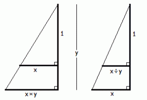
Given line segments x and y, construct (using compass and straight-edge) line segments for the following values:
   x+y
   x-y
   x×y
   x÷y

The first two are immediate. Constructing the last two are straightforward if you are also given 1 (or some other reference length from which to construct 1). Can you construct x×y and x÷y without 1?

Constructing x÷y is impossible if you are not given 1 : From x and y alone you can not determine how they compare to 1. If you can construct x÷y, then you can construct x÷x and therefore relate x and y to 1, contradicting the previous statement.

Can you construct x×y without 1? I got stuck (and lazy) and posed the question to the J Chat Forum, and received a solution from Raul Miller in less than half an hour. Miller’s proof recast in terms similar to that for x÷y is as follows:

From x and y alone you can not determine how they compare to 1. If you can construct x×y, then you can construct x×x, whence:
   if x<x×x then x>1
   if x=x×x then x=1
   if x>x×x then x<1
contradicting the previous statement.

I last thought about this problem in my first year of college many decades ago. At the time Norman M. (a classmate) argued that there must be a 1 and then did the construction for x÷y using 1. I recall he said “there must be a 1” in the sense of “1 has to exist if x and y exist” rather than that “you have to use a 1 in the construction” or “you can not construct x÷y without using 1”. I don’t remember what we did with x×y; before Miller’s message I had some doubt that perhaps we were able to construct x×y without using 1 all those years ago. (Norman went on to get a Ph.D. at MIT and other great things.)

The Story of a Summer Intern

by Suki Tekverk

As a born and raised New Yorker, I thought I had seen it all, but two short weeks spent in Vancouver with Roger Hui and his family proved me very wrong! I went from being at the top of the totem pole to one of the most clueless people around. Luckily, these new experiences provoked new paths of thought and ultimately left me more prepared to face the world than I was when my plane shakily landed in this foreign place.

Upon my arrival, I was greeted by Stella, Roger’s wife, and their children, Nicholas and Rachel, who promptly made me a sign for my bedroom door, making me feel right at home.

The next morning, I went right to work, unsuccessfully writing a dfn for the Fibonacci sequence. After struggling for at least 40 minutes, Roger showed me a solution. This solution was nearly the exact definition of the Fibonacci sequence, setting a precedent for the uncomplicated and direct solutions that ensued. Over the next week we ripped through a Monty Hall simulation, recursive Peano addition and multiplication, recursive and non-recursive binomial coefficients, the Cantor set, the Sierpinski Carpet and more. Over this week, I not only discovered new realms of mathematics but also ate foreign food, hiked through a canyon, watched a Chinese film, made cookies, went to a horse ranch, listened to an orchestra performance, experienced sugar withdrawal and saw a sunset on a mountain. This was just the first week.

The main focus of week two was proofs. At first, I was skeptical of the value of writing proofs in APL as opposed to writing them on paper, but being able to run each step of the proof was quite useful. I started with proof by induction, then by contradiction. After learning the basics I proved the sum of an arithmetic series, sum of geometric series, sum of integers, sum of odd integers and sum of binomial coefficients. This week showed me how closely APL and mathematical notation align. However, I am still annoyed by the fact that the order of operations isn’t how I learnt it in school; it will take some getting used to. My next task will be buying a Windows computer for APL.

Overall, these two weeks in Vancouver were a great learning experience on many levels. Coding in APL has led me to consider possible career options as well as help me understand the nature of the language. Living in a city so far away from home made me question things I considered commonplace and forced me to realize that New York is only a small part of a much larger world.

Loops, Folds and Tuples

For-loops
Given an initial state defined by a number of variables, a for-loop iterates through its argument array modifying the state.

    A←... ⋄ B←... ⋄ C←...       ⍝ initial state
    :For item :In items         ⍝ iterating through array "items"
        A←A ... item            ⍝ new value for A depending on item
        C←C ... A ... item      ⍝ new value for C depending on A and item
        ...                     ⍝ state updated
    :EndFor
    A B C                       ⍝ final state

In the above example the state comprises just three variables. In general, it may be arbitrarily complex, as can the interactions between its various components within the body of the loop.

Dfns
Dfns don’t have for-loops. Instead, we can use reduction (or “fold”) with an accumulating vector “tuple” of values representing the state. Here is the D-equivalent of the above code:

    ⊃{                      ⍝ next item is ⍺
        (A B C)←⍵           ⍝ named items of tuple ⍵
        A∆←A ... ⍺          ⍝ new value for A depending on item ⍺
        C∆←C ... A∆ ... ⍺   ⍝ new value for C depending on A∆ and item ⍺
        ...                 ⍝ ...
        A∆ B C∆             ⍝ "successor" tuple (A and C changed)
    }/(⌽items),⊂A B C       ⍝ for each item and initial state tuple A B C

In this coding, the accumulating tuple arrives as the right argument (⍵) of the operand function, with the next “loop item” on the left (⍺). Notice how the items vector is reversed (⌽items) so that the items arrive in index-order in the right-to-left reduction.

If you prefer your accumulator to be on the left, you can replace the primitive reduction operator (/) with Phil Last’s foldl operator, which also presents its loop items in index-order:

    foldl←{⊃⍺⍺⍨/(⌽⍵),⊂⍺}    ⍝ fold left

then:

    A B C {                 ⍝ final state from initial state (left argument)
        (A B C)←⍺           ⍝ named items of tuple ⍺
        A∆←A ... ⍵          ⍝ new value for A depending on item ⍵
        C∆←C ... A∆ ... ⍵   ⍝ new value for C depending on A∆ and item ⍵
        A∆ B C∆             ⍝ successor tuple (A and C changed)
    } foldl items

If the number of elements in the state tuple is large, it can become unwieldy to name each on entry and exit to the operand function. In this case it simplifies the code to name the indices of the tuple vector, together with an at operator to denote the items of its successor:

    T ← (...) (...) ...         ⍝ intitial state tuple T
    A B C D ... ← ⍳⍴T           ⍝ A B C D ... are tuple item "names"

    T {                         ⍝ final state from initial state (left argument)
        A∆←(A⊃⍺) ... ⍵          ⍝ new value for A depending on item ⍵
        C∆←(C⊃⍺) ... A∆ ... ⍵   ⍝ new value for C depending on A∆ and item ⍵
        A∆ C∆(⊣at A C)⍺         ⍝ successor tuple (A and C changed)
    } foldl items

where:

    at←{A⊣A[⍵⍵]←⍺ ⍺⍺(A←⍵)[⍵⍵]}   ⍝ (⍺ ⍺⍺ ⍵) at ⍵⍵ in ⍵

There is some discussion about providing a primitive operator @ for at in Dyalog V16.

Examples
Function kk illustrates naming tuple elements (S E K Q) at the start of the operand function.
Function scc accesses tuple elements using named indices (C L X x S) and an at operator.

Tuples: a postscript
We might define a “tuple” in APL as a vector in which we think of each item as having a name, rather than an index position.

    bob         ⍝ Tuple: name gender age
┌───┬─┬──┐
│Bob│M│39│
└───┴─┴──┘

    folk        ⍝ Vector of tuples
┌──────────┬────────────┬──────────┬────────────┬─
│┌───┬─┬──┐│┌─────┬─┬──┐│┌───┬─┬──┐│┌─────┬─┬──┐│
││Bob│M│39│││Carol│F│31│││Ted│M│31│││Alice│F│32││ ...
│└───┴─┴──┘│└─────┴─┴──┘│└───┴─┴──┘│└─────┴─┴──┘│
└──────────┴────────────┴──────────┴────────────┴─

    ↓⍉↑ folk    ⍝ Tuple of vectors
┌─────────────────────────┬────────┬───────────────┐
│┌───┬─────┬───┬─────┬─   │MFMF ...│39 31 31 32 ...│
││Bob│Carol│Ted│Alice│ ...│        │               │
│└───┴─────┴───┴─────┴─   │        │               │
└─────────────────────────┴────────┴───────────────┘

    ⍪∘↑¨ ↓⍉↑ folk   ⍝ Tuple of matrices
┌─────┬─┬──┐
│Bob  │M│39│
│Carol│F│31│
│Ted  │M│31│
│Alice│F│32│
 ...   . ..
└─────┴─┴──┘

APLers sometimes talk about “inverted files”. In this sense, a “regular” file is a vector-of-tuples and an inverted file (or more recently: “column store”) is a tuple-of-vectors (or matrices).