Selective Expression Tracing

Operator trace from dfns.dws is a simple and low-tech tool for displaying intermediate results of functions, during the evaluation of an expression. For example, what’s going on here?

      (+⌿ ÷ ≢) 1 2 3 4
2.5

We can guess that the above fork is computing the average of the right argument. To see how this works:

      )copy dfns trace
...

⍝ Rename to reduce clutter

      t ← trace

⍝ Bind each "tine" of the fork with t to see what's happening

      (+⌿t ÷t ≢t) 1 2 3 4
≢  1 2 3 4  =>  4
+⌿  1 2 3 4  =>  10
10  ÷  4  =>  2.5
2.5

⍝ But how is that +⌿ reduction evaluated?

      (+t⌿ ÷ ≢) 1 2 3 4
3  +  4  =>  7
2  +  7  =>  9
1  +  9  =>  10
2.5

As a second example, what does the atop (~⍷) do in the following function to remove superfluous '.' characters from its argument?

      {('··'(~⍷)⍵)/⍵} 'squeeze·····me'
squeeze·me

      {('··'(~⍷)t⍵)/⍵} 'squeeze·····me'
··  ~⍷  squeeze·····me  =>  1 1 1 1 1 1 1 0 0 0 0 1 1 1
squeeze·me

…and so forth. Notice how t can be injected to the right of any of the functions in an expression.

For more examples, see the notes for trace.

Data-driven Conditionals

ACKNOWLEDGEMENT: My thanks to Andy Shiers for simplifying the examples

Visitors to APL from other languages are sometimes a bit sniffy about our use of numbers (1 0) for Boolean values True and False. They’re further bemused by our fondness for moving conditional processing out of code and into data. For example, instead of:

   0=2|⍵: ⍵÷2 ⋄ ⍵       ⍝ even number: half

we might say:

   ⍵ ÷ 1+0=2|⍵          ⍝ half if even

At first blush, this seems a bit loony; such transformations appear to produce code which is both slower and more obscure! Here’s another example:

   2|⍵: 1+3×⍵ ⋄ ⍵       ⍝ odd: one more than its triple

vs:

   p ← 2|⍵              ⍝ parity
   p + ⍵ × 1+2×p        ⍝ one more than triple, if odd

But think arrays! Data-driven processing of conditionals is inherently parallel and so performs significantly better for large arrays.

The Collatz conjecture asserts that the sequence “half if even, else one plus triple if odd” always converges to 1. For example, for the number 7 this sequence is:

   7 22 11 34 17 52 26 13 40 20 10 5 16 8 4 2 1

To test this up to a million we can borrow time, a coarse-grained timing operator, from dfns.dws:

      scalar←{                                  
          {                 ⍝ scalar function
              2|⍵:1+3×⍵     ⍝ odd              
              ⍵÷2           ⍝ even             
          }⍣{⍺=1}¨⍵         ⍝ applied under each
      }


      vector←{         
          {                 ⍝ vector function                                              
              p←2|⍵         ⍝ parity                   
              u←⍵÷2-p       ⍝ half of evens            
              v←p+u×1+2×p   ⍝ 1+3× odds                
              ∪v~1          ⍝ without 1s and duplicates
          }⍣{⍺≡⍬}⍵          ⍝ applied to whole vector                           
      }  


      scalar time ⍳1e6      ⍝ scalar processing 8¾ minutes
08:46.03
 
      vector time ⍳1e6      ⍝ array processing 8¾ seconds
08.74

In the above, time and are high order “operators”.

Defined operator time takes a function left operand, which it applies to its argument, returning the execution time in minutes and seconds.

Primitive operator (power or fixpoint) applies its left operand function repeatedly until its right operand function, which is supplied with the result () and argument of each application, returns True (1).

For further discussion of the Collatz function, see http://dfns.dyalog.com/n_osc.htm.

Why Dyalog ’14 was a Shear Delight

rot55

Recent versions of Microsoft Windows support touch screens, which of course means that applications can respond to events originating from touches. Microsoft calls these events “gestures”.

Dyalog decided to add support for gestures to version 14.1 and so projects were planned, designs were designed, code was coded and, at Dyalog ’14 (#Dyalog14), a demonstration was demonstrated. The video of that demonstration is here

The three most interesting gestures are “pan”, “zoom” and “rotate”; I needed a good demo for the rotate gesture. I had an idea but was unsure how to implement it, so I decided to ask the team. Here’s the email I sent (any typos were included in the original email!):

“Does any have code (or an algorithm, but code ‘d be better) to rotate a matrix by an arbitrary angle. The resulting matrix may then be larger than the original but will be filled with an appropriate value.
Does the question makes sense? For the conference I want to demonstrate 14.1 support for Windows touch gestures, one of which is a “rotate” gesture, and I thought that a good demo would be to rotate a CD cover image when the gesture is detected. So I need to be able to rotate the RGB values that make up the image.”

There were a number of helpful responses, mainly about using rotation matrices, but what intrigued me was Jay Foad’s almost throw away comment: “It’s also possible to do a rotation with repeated shears”

That looked interesting, so I had a bit of a Google and found an article on rotation by shearing written by Tobin Fricke. The gist of this article is that shearing a matrix three times (first horizontally, then vertically and then again horizontally) effects a rotation. An interesting aspect of this (as compared to the rotation method) is that no information is lost. Every single pixel is moved and there is no loss of quality of the image.

I’m no mathematician, but I could read my way though enough of that to realise that it would be trivial in APL. The only “real” code needed is to figure how much to shear each line in the matrix.

Converting Fricke’s α=-tan(Θ/2) and ϐ=sin(Θ), we get (using for Θ):

a←-3○⍺÷2
b←1○⍺

and so, for a given matrix, the amounts to shift are given by:

⌊⍺×(⍳≢⍵)-0.5×≢⍵

where is either a or b, depending on which shift we are doing.

Wrapping this in an operator (where ⍺⍺ is either or ):

shear←{
(⌊⍺×(⍳≢⍵)-0.5×≢⍵)⍺⍺ ⍵
}

Our three shears of matrix , of size s, can therefore be written as:

a⌽shear b⊖shear a⌽shear(3×s)↑(-2×s)↑⍵

Note the resize and pad of the matrix before we start so that we don’t replicate the edges of the bitmap. The padding elements are zeros and display as black pixels. They have been removed from the images below for clarity.

The final rotate function is:

rotate←{
shear←{(⌊⍺×(⍳≢⍵)-0.5×≢⍵)⍺⍺ ⍵}
a←-3○⍺÷2 ⋄ b←1○⍺ ⋄ s←⍴⍵
a⌽shear b⊖shear a⌽shear(3×s)↑(-2×s)↑⍵
}

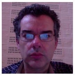
Let’s look at a 45° rotate of a bitmap called “jd”.

jd.CBits←(○.25)rotate jd.CBits

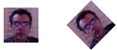
Prior to performing any shears our image is:

rot0

After the first shear it becomes:

rot1

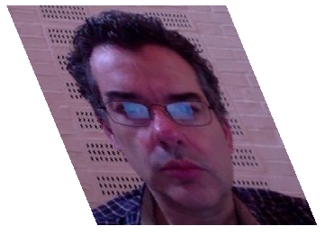
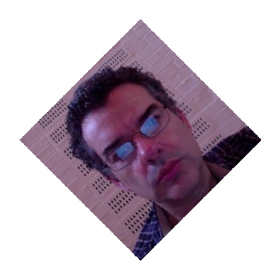
After the second shear it is:

rot2

And after the third shear it is:

rot3

All nicely rotated.