Towards Improvements to Stencil

Background

The stencil operator was introduced in Dyalog version 16.0 in 2017. Recently we received some feedback (OK, complaints) that (a) stencil does padding which is unwanted sometimes and needs to be removed from the result and (b) stencil is too slow when it is not supported by special code.

First, stencil in cases supported by special code is much faster than when it is not. The special cases are as follows, from Dyalog ’17 Workshop SA3.

   {⍵}      {⊢⍵}      {,⍵}      {⊂⍵}
{+/,⍵}    {∧/,⍵}    {∨/,⍵}    {=/,⍵}    {≠/,⍵}  
    
{  +/,A×⍵}    {  +/⍪A×⍤2⊢⍵}
{C<+/,A×⍵}    {C<+/⍪A×⍤2⊢⍵}
C:  a single number or variable whose value is a single number
A:  a variable whose value is a rank-2 or 3 array
The comparison can be < ≤ ≥ > = ≠
odd window size; movement 1; matrix argument
 

You can test whether a particular case is supported by using a circumlocution to defeat the special case recognizer.

   )copy dfns cmpx

   cmpx '{⍵}⌺3 5⊢y' '{⊢⊢⍵}⌺3 5⊢y' ⊣ y←?100 200⍴0
  {⍵}⌺3 5⊢x   → 4.22E¯4 |      0%                               
  {⊢⊢⍵}⌺3 5⊢x → 5.31E¯2 | +12477% ⎕⎕⎕⎕⎕⎕⎕⎕⎕⎕⎕⎕⎕⎕⎕⎕⎕⎕⎕⎕⎕⎕⎕⎕⎕⎕⎕⎕⎕⎕

   cmpx '{⌽⍵}⌺3 5⊢y' '{⊢⊢⌽⍵}⌺3 5⊢y'
  {⌽⍵}⌺3 5⊢y   → 2.17E¯1 |  0% ⎕⎕⎕⎕⎕⎕⎕⎕⎕⎕⎕⎕⎕⎕⎕⎕⎕⎕⎕⎕⎕⎕⎕⎕⎕⎕⎕⎕⎕⎕
  {⊢⊢⌽⍵}⌺3 5⊢y → 2.21E¯1 | +1% ⎕⎕⎕⎕⎕⎕⎕⎕⎕⎕⎕⎕⎕⎕⎕⎕⎕⎕⎕⎕⎕⎕⎕⎕⎕⎕⎕⎕⎕⎕

If the timings are the same then there is no special code.

Padding and performance improvements will take a lot of work. For example, for padding (i.e. the treatment of cells at the edge of the universe) multiple options are possible: no padding, padding, wrap from opposite edge, etc. While working on these improvements I hit upon the idea of writing a stencil function which produces the stencil cells. It only works with no padding and only for movements of 1 (which I understand are common cases), but turns out to be an interesting study.

A Stencil Function

⍺ stencell ⍵ produces the stencil cells of size from  , and is equivalent to {⍵}⌺⍺⊢⍵ after the padded cells are removed.

stencell←{
  ⎕io←0                 ⍝ ⎕io delenda est!
  s←(≢⍺)↑⍴⍵
  f←1+s-⍺               ⍝ frame AKA outer shape
  m←⊖×⍀⊖1↓s,1           ⍝ multiplier for each axis
  i←⊃∘.+⌿(m,m)×⍳¨f,⍺    ⍝ indices
  (⊂i) ⌷ ⍵ ⍴⍨ (×⌿(≢⍺)↑⍴⍵),(≢⍺)↓⍴⍵
}

For example, stencell is applied to x with cell shape 3 5 .

   ⊢ x←6 10⍴⍳60                    ⍝ (a)
 0  1  2  3  4  5  6  7  8  9
10 11 12 13 14 15 16 17 18 19
20 21 22 23 24 25 26 27 28 29
30 31 32 33 34 35 36 37 38 39
40 41 42 43 44 45 46 47 48 49
50 51 52 53 54 55 56 57 58 59

   c←3 5 stencell x                ⍝ (b)
   ⍴c
4 6 3 5

   c ≡ 1 2 ↓ ¯1 ¯2 ↓ {⍵}⌺3 5 ⊢x    ⍝ (c)
1

   ⊢ e←⊂⍤2 ⊢c                      ⍝ (d)
┌──────────────┬──────────────┬──────────────┬──────────────┬──────────────┬──────────────┐
│ 0  1  2  3  4│ 1  2  3  4  5│ 2  3  4  5  6│ 3  4  5  6  7│ 4  5  6  7  8│ 5  6  7  8  9│
│10 11 12 13 14│11 12 13 14 15│12 13 14 15 16│13 14 15 16 17│14 15 16 17 18│15 16 17 18 19│
│20 21 22 23 24│21 22 23 24 25│22 23 24 25 26│23 24 25 26 27│24 25 26 27 28│25 26 27 28 29│
├──────────────┼──────────────┼──────────────┼──────────────┼──────────────┼──────────────┤
│10 11 12 13 14│11 12 13 14 15│12 13 14 15 16│13 14 15 16 17│14 15 16 17 18│15 16 17 18 19│
│20 21 22 23 24│21 22 23 24 25│22 23 24 25 26│23 24 25 26 27│24 25 26 27 28│25 26 27 28 29│
│30 31 32 33 34│31 32 33 34 35│32 33 34 35 36│33 34 35 36 37│34 35 36 37 38│35 36 37 38 39│
├──────────────┼──────────────┼──────────────┼──────────────┼──────────────┼──────────────┤
│20 21 22 23 24│21 22 23 24 25│22 23 24 25 26│23 24 25 26 27│24 25 26 27 28│25 26 27 28 29│
│30 31 32 33 34│31 32 33 34 35│32 33 34 35 36│33 34 35 36 37│34 35 36 37 38│35 36 37 38 39│
│40 41 42 43 44│41 42 43 44 45│42 43 44 45 46│43 44 45 46 47│44 45 46 47 48│45 46 47 48 49│
├──────────────┼──────────────┼──────────────┼──────────────┼──────────────┼──────────────┤
│30 31 32 33 34│31 32 33 34 35│32 33 34 35 36│33 34 35 36 37│34 35 36 37 38│35 36 37 38 39│
│40 41 42 43 44│41 42 43 44 45│42 43 44 45 46│43 44 45 46 47│44 45 46 47 48│45 46 47 48 49│
│50 51 52 53 54│51 52 53 54 55│52 53 54 55 56│53 54 55 56 57│54 55 56 57 58│55 56 57 58 59│
└──────────────┴──────────────┴──────────────┴──────────────┴──────────────┴──────────────┘

    ∪¨ ,¨ e-⍬⍴e                    ⍝ (e)
┌──┬──┬──┬──┬──┬──┐
│0 │1 │2 │3 │4 │5 │
├──┼──┼──┼──┼──┼──┤
│10│11│12│13│14│15│
├──┼──┼──┼──┼──┼──┤
│20│21│22│23│24│25│
├──┼──┼──┼──┼──┼──┤
│30│31│32│33│34│35│
└──┴──┴──┴──┴──┴──┘
(a)  The matrix x is chosen to make stencil results easier to understand.
(b) stencell is applied to x with cell shape 3 5 .
(c) The result of stencell is the same as that for {⍵}⌺ after cells with padding are dropped.
(d) Enclose the matrices in c (the cells) to make the display more compact and easier to understand.
(e) Subsequent discussion is based on the observation that each cell is some scalar integer added to the first cell.

Indices

The key expression in the computation is

   ⊃∘.+⌿(m,m)×⍳¨f,⍺ 

where

   m:  10 1;  multiplier for each axis
   f:  4 6;  multiplier for each axis
   ⍺:  3 5;  multiplier for each axis
 

We discuss a more verbose but equivalent version of this expression,

   (⊃∘.+⌿m×⍳¨f)∘.+(⊃∘.+⌿m×⍳¨⍺)

and in particular the right half, ⊃∘.+⌿m×⍳¨⍺ , which produces the first cell.

   ⍳⍺               ⍝ ⍳3 5
┌───┬───┬───┬───┬───┐
│0 0│0 1│0 2│0 3│0 4│
├───┼───┼───┼───┼───┤
│1 0│1 1│1 2│1 3│1 4│
├───┼───┼───┼───┼───┤
│2 0│2 1│2 2│2 3│2 4│
└───┴───┴───┴───┴───┘
   (⍴⍵)∘⊥¨⍳⍺        ⍝ 6 10∘⊥¨ ⍳3 5
 0  1  2  3  4
10 11 12 13 14
20 21 22 23 24

Alternatively, this last result obtains by multiplying by m the corresponding indices for each axis, where an element of m is the increment for a unit in an axis. That is, m←⊖×⍀⊖1↓s,1 where s←(≢⍺)↑⍴⍵ is a prefix of the shape of  . The multipliers are with respect to the argument because the indices are required to be with respect to the argument  .

   ⍳¨⍺              ⍝ ⍳¨3 5
┌─────┬─────────┐
│0 1 2│0 1 2 3 4│
└─────┴─────────┘
   m×⍳¨⍺            ⍝ 10 1×⍳¨3 5
┌───────┬─────────┐
│0 10 20│0 1 2 3 4│
└───────┴─────────┘
   ∘.+⌿ m×⍳¨⍺       ⍝ ∘.+⌿ 10 1×⍳¨3 5
┌──────────────┐
│ 0  1  2  3  4│
│10 11 12 13 14│
│20 21 22 23 24│
└──────────────┘
   ((⍴⍵)∘⊥¨⍳⍺) ≡ ⊃∘.+⌿m×⍳¨⍺
1

This alternative computation is more efficient because it avoids creating and working on lots of small nested vectors and because the intermediate results for ∘.+⌿ grows fast from one to the next (i.e., O(⍟n) iterations in the main loop).

The left half, ⊃∘.+⌿m×⍳¨f , is similar, and computes the necessary scalar integers to be added to the result of the right half.

   ⊃ ∘.+⌿ m×⍳¨f     ⍝ ⊃ ∘.+⌿ 10 1×⍳¨4 6
 0  1  2  3  4  5
10 11 12 13 14 15
20 21 22 23 24 25
30 31 32 33 34 35

The shorter expression derives from the more verbose one by some simple algebra.

(⊃∘.+⌿m×⍳¨f)∘.+(⊃∘.+⌿m×⍳¨⍺)    ⍝ verbose version
⊃∘.+⌿(m×⍳¨f),m×⍳¨⍺             ⍝ ∘.+ is associative
⊃∘.+⌿(m,m)×(⍳¨f),⍳¨⍺           ⍝ m× distributes over ,
⊃∘.+⌿(m,m)×⍳¨f,⍺               ⍝ ⍳¨ distributes over ,

I am actually disappointed that the shorter expression was found ☺; it would have been amusing to have a non-contrived and short expression with three uses of ∘.+ .

Cells

Having the indices i in hand, the stencil cells obtain by indexing into an appropriate reshape or ravel of the right argument  . In general, the expression is

   (⊂i) ⌷ ⍵ ⍴⍨ (×/(≢⍺)↑⍴⍵),(≢⍺)↓⍴⍵

specifies the cell shape. If (≢⍺)=≢⍴⍵ , that is, if a length is specified for each axis of  , the expression is equivalent to (⊂i)⌷,⍵ or (,⍵)[i] ; if (≢⍺)<≢⍴⍵ , that is, if there are some trailing unstencilled axes, the expression is equivalent to (,[⍳≢⍺]⍵)[i;…;] (the leading ≢⍺ axes are ravelled) or ↑(,⊂⍤((≢⍴⍵)-≢⍺)⊢⍵)[i] (as if the trailing axes were shielded from indexing). The general expression covers both cases.

Application

stencell makes it possible to workaround current shortcomings in . The alternative approach is to use stencell to get all the stencil cells, all at once, and then work on the cells using  , +.× , and
other efficient primitives.

The following example is from Aaron Hsu. In the original problem the size of x is 512 512 64 .

   K←?64 3 3 64⍴0
   x←?256 256 64⍴0

   t←1 1↓¯1 ¯1↓{+/⍪K×⍤3⊢⍵}⌺3 3⊢x
   ⍴t
256 256 64

   cmpx '1 1↓¯1 ¯1↓{+/⍪K×⍤3⊢⍵}⌺3 3⊢x'
6.76E0 

The computation is slow because the cells are rank-3, not supported by special code. Aaron then devised a significant speed-up using a simpler left operand to create the ravels of the cells (but still no special code):

   t ≡ (1 1↓¯1 ¯1↓{,⍵}⌺3 3⊢x)+.×⍉⍪K
1
   cmpx '(1 1↓¯1 ¯1↓{,⍵}⌺3 3⊢x)+.×⍉⍪K'
1.67E0 

Use of stencell would improve the performance a bit further:

   t ≡ (,⍤3 ⊢3 3 stencell x)+.×⍉⍪K
1
   cmpx '(,⍤3 ⊢3 3 stencell x)+.×⍉⍪K'
1.09E0 

   cmpx '3 3 stencell x'
6.10E¯2

The last timing shows that the stencell computation is 6% (6.10e¯2÷1.09e0) of the total time.

Materializing all the cells does take more space than if the computation is incorporated in the left operand of  , and is practicable only if the workspace sufficiently large.

   )copy dfns wsreq

   wsreq '1 1↓¯1 ¯1↓{+/⍪K×⍤3⊢⍵}⌺3 3⊢x'
110649900
   wsreq '(1 1↓¯1 ¯1↓{,⍵}⌺3 3⊢x)+.×⍉⍪K'
647815900
   wsreq '(,⍤3 ⊢3 3 stencell x)+.×⍉⍪K'
333462260

Performance

stencell is competitive with {⍵}⌺ on matrices, where it is supported by special code written in C, and is faster when there is no special code. The benchmarks are done on a larger argument to reduce the effects of padding/unpadding done in {⍵}⌺ .

   y2←?200 300⍴0
          
   cmpx '3 5 stencell y2' '1 2↓¯1 ¯2↓{⍵}⌺3 5⊢y2' 
  3 5 stencell y      → 1.85E¯3 |   0% ⎕⎕⎕⎕⎕⎕⎕⎕⎕⎕⎕⎕⎕⎕⎕⎕⎕⎕⎕           
  1 2↓¯1 ¯2↓{⍵}⌺3 5⊢y → 2.91E¯3 | +57% ⎕⎕⎕⎕⎕⎕⎕⎕⎕⎕⎕⎕⎕⎕⎕⎕⎕⎕⎕⎕⎕⎕⎕⎕⎕⎕⎕⎕⎕⎕

   cmpx '3 5 stencell y' '{⍵}⌺3 5⊢y' 
  3 5 stencell y → 1.85E¯3 |   0% ⎕⎕⎕⎕⎕⎕⎕⎕⎕⎕⎕⎕⎕⎕⎕⎕⎕⎕⎕⎕⎕⎕⎕⎕⎕⎕⎕⎕⎕⎕
* {⍵}⌺3 5⊢y      → 1.04E¯3 | -45% ⎕⎕⎕⎕⎕⎕⎕⎕⎕⎕⎕⎕⎕⎕⎕⎕⎕             

   y3←?200 300 64⍴0

   cmpx '3 5 stencell y3' '1 2↓¯1 ¯2↓{⍵}⌺3 5⊢y3' 
  3 5 stencell y3      → 8.90E¯2 |    0% ⎕⎕⎕                           
  1 2↓¯1 ¯2↓{⍵}⌺3 5⊢y3 → 7.78E¯1 | +773% ⎕⎕⎕⎕⎕⎕⎕⎕⎕⎕⎕⎕⎕⎕⎕⎕⎕⎕⎕⎕⎕⎕⎕⎕⎕⎕⎕⎕⎕⎕

   cmpx '3 5 stencell y3' '{⍵}⌺3 5⊢y3' 
  3 5 stencell y3 → 9.38E¯2 |    0% ⎕⎕⎕⎕⎕⎕⎕⎕                      
* {⍵}⌺3 5⊢y3      → 3.34E¯1 | +256% ⎕⎕⎕⎕⎕⎕⎕⎕⎕⎕⎕⎕⎕⎕⎕⎕⎕⎕⎕⎕⎕⎕⎕⎕⎕⎕⎕⎕⎕⎕

There is an interesting question of whether the shorter version of the key computation (in the Indices section above) is faster than the more verbose version.

   m←10 1 ⋄ f←4 6 ⋄ a←3 5

   cmpx '⊃∘.+⌿(m,m)×⍳¨f,a' '(⊃∘.+⌿m×⍳¨f)∘.+(⊃∘.+⌿m×⍳¨a)'
  ⊃∘.+⌿(m,m)×⍳¨f,a            → 3.75E¯6 |   0% ⎕⎕⎕⎕⎕⎕⎕⎕⎕⎕⎕⎕⎕⎕⎕⎕⎕⎕⎕
  (⊃∘.+⌿m×⍳¨f)∘.+(⊃∘.+⌿m×⍳¨a) → 5.20E¯6 | +38% ⎕⎕⎕⎕⎕⎕⎕⎕⎕⎕⎕⎕⎕⎕⎕⎕⎕⎕⎕⎕⎕⎕⎕⎕⎕⎕

In this case, it is faster, and I expect it will be faster for cases which arise in stencil calculations, where the argument size is larger than the cell size. But it is easy to think of arguments where ∘.+⌿ is slower than ∘.+ done with a different grouping:

   cmpx '((⍳0)∘.+⍳100)∘.+⍳200' '(⍳0)∘.+((⍳100)∘.+⍳200)' '⊃∘.+/⍳¨0 100 200'
  ((⍳0)∘.+⍳100)∘.+⍳200   → 7.86E¯7 |     0% ⎕⎕                            
  (⍳0)∘.+((⍳100)∘.+⍳200) → 1.05E¯5 | +1234% ⎕⎕⎕⎕⎕⎕⎕⎕⎕⎕⎕⎕⎕⎕⎕⎕⎕⎕⎕⎕⎕⎕⎕⎕⎕⎕⎕⎕  
  ⊃∘.+/⍳¨0 100 200       → 1.11E¯5 | +1310% ⎕⎕⎕⎕⎕⎕⎕⎕⎕⎕⎕⎕⎕⎕⎕⎕⎕⎕⎕⎕⎕⎕⎕⎕⎕⎕⎕⎕⎕⎕

This question will be explored further in a later post.

Ascending and Descending

Lexicographic Ordering

Lexicographic ordering is what the APL primitives and provide:

   ⎕io←0     ⍝ ⎕io delenda est
   ⎕rl←7*5   ⍝ to get reproducible random results

   a←?11 3⍴3

   a          a ⌷⍨⊂ ⍋a
2 1 0      0 1 0
0 2 2      0 2 2
1 1 1      1 0 0
1 0 0      1 0 1
1 1 1      1 0 1
1 2 1      1 1 0
1 0 1      1 1 1
1 0 1      1 1 1
1 1 0      1 2 1
0 1 0      1 2 2
1 2 2      2 1 0

First order by column 0, resulting in groups of rows with the same values in column 0. Then, within each group, order by column 1, getting subgroups with the same values in columns 0 and 1. Then, within each subgroup, order by column 2, getting subsubgroups with the same values in columns 0, 1, and 2. In general, for each subsub…subgroup, order by column k, getting groups with identical values in columns ⍳k.

The preceding discourse is descriptive rather than prescriptive—algorithms for can use more efficient and more straightforward approaches. As well, for ease of understanding, the description is for a matrix and speaks of columns and rows. In general, any non-scalar array can be ordered, whence instead of rows, think major cells, instead of column, think item in a major cell. Symbolically and more succinctly, ⍋⍵ ←→ ⍋⍪⍵.

can be used if the orderings in the process are all ascending, or if all descending. The problem to be solved here is where the orderings are a mix of ascending and descending.

Numeric Arrays

Since ⍒⍵ ←→ ⍋-⍵ if is numeric, for such multiply each descending column by ¯1 and each ascending column by 1, then apply . This induces a “control array” having the same shape as a major cell of the argument, with a ¯1 for descending and a 1 for ascending.

   adn←{⍵ ⌷⍨⊂ ⍋ ⍺ ×⍤99 ¯1 ⊢⍵}

For the array a in the previous section:

   a              1 ¯1 1 adn a        ¯1 1 1 adn a
2 1 0          0 2 2               2 1 0  
0 2 2          0 1 0               1 0 0  
1 1 1          1 2 1               1 0 1  
1 0 0          1 2 2               1 0 1  
1 1 1          1 1 0               1 1 0  
1 2 1          1 1 1               1 1 1  
1 0 1          1 1 1               1 1 1  
1 0 1          1 0 0               1 2 1  
1 1 0          1 0 1               1 2 2  
0 1 0          1 0 1               0 1 0  
1 2 2          2 1 0               0 2 2  

In 1 ¯1 1 adn a, column 0 is ascending, and within that, column 1 is descending, and within that, column 2 is ascending. In ¯1 1 1 adn a, column 0 is descending, and within that, column 1 is ascending, and within that, column 2 is ascending.

Ordinals

An array to be sorted can be converted to an order-equivalent integer array by assigning to each item an ordinal (an integer) which has the same ordering relationship as the original item relative to other items in the array:

   sort    ← {(⊂⍋⍵)⌷⍵}
   ordinal ← {⎕ct←0 ⋄ ⍵⍳⍨sort,⍵}

That is, the ordinals obtain as the indices of the original array in the sorted list of the ravelled elements, using exact comparisons. (Exact comparisons are used because sorting necessarily uses exact comparisons.)
For example:

   ⊢ d←¯1 'syzygy' (3 ¯5) 1j2 'chthonic' (¯1)
┌──┬──────┬────┬───┬────────┬──┐
│¯1│syzygy│3 ¯5│1J2│chthonic│¯1│
└──┴──────┴────┴───┴────────┴──┘
   ordinal d
0 5 3 2 4 0

In the example, the data items are ¯1, 'syzygy', 'chthonic', 3 ¯5, 1j2, and ¯1 again. With respect to ordering, these data items are perfectly represented by the ordinals (numbers) 0, 5, 3, 2, 4, and 0, respectively. That is, ⍋d ←→ ⍋ordinal d.

   ⍋ d
0 5 3 2 4 1
   ⍋ ordinal d
0 5 3 2 4 1

As the example illustrates, it is imperative that identical ordinals are assigned to identical items, else the ordering relationships would be changed. For example, if b←0,⍪2 1 and the 0s are assigned different ordinals,

   ⊢ b←0,⍪2 1               
0 2
0 1
   ordinal b                 ⊢ bo←0 3,⍪1 2  ⍝ faux ordinals
0 3                       0 3
0 2                       1 2
   ⍋ ordinal b               ⍋ bo
1 0                       0 1
   ⍋ b
1 0

Computation of ordinals is greatly facilitated by the total array ordering introduced in Dyalog APL version 17.0.

Non-Numeric Arrays

A general solution for the ordering problem obtains by first converting the array to an order-equivalent integer array through the use of ordinals.

   ado ← {⍵ ⌷⍨⊂ ⍋ ⍺ ×⍤99 ¯1 ordinal ⍵}

For example:

   ⎕rl←7*5   ⍝ to get reproducible random results

   x0← ?19⍴4                            
   x1← (⊂?19⍴2) ⌷ 'alpha' 'beta'          
   x2← (⊂?19⍴3) ⌷ 'abc'                   
   x3← (⊂?19⍴3) ⌷ 'able' 'baker' 'charlie'

   x ← x0,x1,x2,⍪x3

   ordinal x
13 49 19 42
10 49 32 68
13 49 63 68
 4 49 63 42
 0 27 19 23
13 49 32 42
 0 49 19 42
10 49 32 68
10 27 32 23
 4 49 32 68
 4 49 32 68
 4 27 32 23
 4 49 32 68
 0 49 63 68
13 49 63 68
 0 49 32 42
13 27 32 23
 4 27 63 42
13 49 19 42

   (⍋x) ≡ ⍋ ordinal x
1

Suppose x is to be sorted ascending in columns 0 and 2 and descending in columns 1 and 3. The control array is 1 ¯1 1 ¯1, and:

   x                       1 ¯1 1 ¯1 ado x
┌─┬─────┬─┬───────┐     ┌─┬─────┬─┬───────┐
│2│beta │b│baker  │     │0│beta │a│able   │
├─┼─────┼─┼───────┤     ├─┼─────┼─┼───────┤
│3│alpha│a│able   │     │0│beta │b│charlie│
├─┼─────┼─┼───────┤     ├─┼─────┼─┼───────┤
│3│beta │b│able   │     │0│beta │b│baker  │
├─┼─────┼─┼───────┤     ├─┼─────┼─┼───────┤
│3│alpha│b│baker  │     │0│beta │c│charlie│
├─┼─────┼─┼───────┤     ├─┼─────┼─┼───────┤
│1│beta │b│charlie│     │0│beta │c│able   │
├─┼─────┼─┼───────┤     ├─┼─────┼─┼───────┤
│1│beta │a│baker  │     │0│alpha│c│baker  │
├─┼─────┼─┼───────┤     ├─┼─────┼─┼───────┤
│0│beta │c│charlie│     │1│beta │a│baker  │
├─┼─────┼─┼───────┤     ├─┼─────┼─┼───────┤
│0│beta │b│baker  │     │1│beta │b│charlie│
├─┼─────┼─┼───────┤     ├─┼─────┼─┼───────┤
│0│beta │c│able   │     │1│alpha│c│able   │
├─┼─────┼─┼───────┤     ├─┼─────┼─┼───────┤
│0│beta │a│able   │     │2│beta │a│baker  │
├─┼─────┼─┼───────┤     ├─┼─────┼─┼───────┤
│3│alpha│a│baker  │     │2│beta │b│baker  │
├─┼─────┼─┼───────┤     ├─┼─────┼─┼───────┤
│3│alpha│a│baker  │     │3│beta │b│able   │
├─┼─────┼─┼───────┤     ├─┼─────┼─┼───────┤
│1│alpha│c│able   │     │3│beta │b│able   │
├─┼─────┼─┼───────┤     ├─┼─────┼─┼───────┤
│0│beta │b│charlie│     │3│beta │c│charlie│
├─┼─────┼─┼───────┤     ├─┼─────┼─┼───────┤
│0│alpha│c│baker  │     │3│alpha│a│baker  │
├─┼─────┼─┼───────┤     ├─┼─────┼─┼───────┤
│3│beta │b│able   │     │3│alpha│a│baker  │
├─┼─────┼─┼───────┤     ├─┼─────┼─┼───────┤
│2│beta │a│baker  │     │3│alpha│a│able   │
├─┼─────┼─┼───────┤     ├─┼─────┼─┼───────┤
│3│beta │c│charlie│     │3│alpha│a│able   │
├─┼─────┼─┼───────┤     ├─┼─────┼─┼───────┤
│3│alpha│a│able   │     │3│alpha│b│baker  │
└─┴─────┴─┴───────┘     └─┴─────┴─┴───────┘

Finally

   (ordinal x) ≡ ordinal ordinal x
1

That is, ordinal is idempotent. Actually, this is kind of obvious, but I never miss an opportunity to use the word “idempotent”.☺

Krypto

In the 2016 Year Game, the task was to generate the numbers 0 to 100 using APL primitives and the digits 2 0 1 6 in that order. For example,

   20=16
   ×2016
   2⌊016
   2+×016
   …

This “puzzle of the year” brings to mind Krypto, a game I played many years ago while in grade school.

Krypto

Krypto is a mathematical card game. The Krypto deck has 56 cards: 3 each of numbers 1-6, 4 each of the numbers 7-10, 2 each of 11-17, 1 each of 18-25.

   ⎕io←0
   DECK ← (3/1+⍳6),(4/7+⍳4),(2/11+⍳7),18+⍳8

Six cards are dealt: an objective card and five other cards. A player must use all five of the latter cards’ numbers exactly once, using any combination of arithmetic operations (+, -, ×, and ÷) to form the objective card’s number. The first player to come up with a correct formula is the winner. The stricter “International Rules” specify the use of non-negative integers only; fractional or negative intermediate results are not permitted.

For example, if the objective card were 17 and the other cards were 2, 8, 14, 19, and 21, then a Krypto solution can be as follows. Without loss of generality, we use APL notation and syntax.

   8 - 19 + 14 - 2 × 21

In this article we present functions to find all solutions to a Krypto hand.

A Solution

There are a maximum of !5 permutations of the 5 cards and 4 possibilities in each of the 4 places where an operation can be put, for (!5)×4*4 or 30720 total possibilities. This number is small enough for an exhaustive approach.

deal←{DECK ⌷⍨⊂ 6?≢DECK}

Krypto←{
  perm←{0=⍵:1 0⍴0 ⋄ ,[⍳2](⊂0,1+∇ ¯1+⍵)⌷⍤1⍒⍤1∘.=⍨⍳⍵}
  a←256⌿5 0⍕⍵[perm 5]
  a[;6+5×⍳4]←'+-×÷'[((256×!5),4)⍴⍉(4⍴4)⊤⍳256]
  ⊣⌸ a ⌿⍨ ⍺ = ⍎⍤1 ⊢a
}

   deal ⍬
17 8 19 14 2 21

   ⊢ t← 17 Krypto 8 19 14 2 21
    8 - 19 + 14 -  2 × 21
    8 - 19 + 14 - 21 ×  2
    8 - 19 - 21 + 14 ÷  2
    8 - 14 + 19 -  2 × 21
        ...
   21 +  8 - 19 - 14 ÷  2
   21 - 19 -  8 + 14 ÷  2

   ⍴ t
24 25

Intermediate Steps

The function perm is from the Dyalog blog post Permutations, 2015-07-20. perm n generates the sorted table of all permutations of ⍳n.

The local variable a in Krypto is a 30720-row character matrix computed from the 5 non-objective numbers. It consists of all !5 permutations of the 5 numbers interspersed with all 4*4 arrangements of the four operations + - × ÷.

Executing the rows of a produces a 30720-element numeric vector. Comparison of this vector with the objective yields a boolean vector that selects the rows of a which are correct formulas.

   ⍴ a
30720 25

   8↑a
    8 + 19 + 14 +  2 + 21
    8 + 19 + 14 +  2 - 21
    8 + 19 + 14 +  2 × 21
    8 + 19 + 14 +  2 ÷ 21
    8 + 19 + 14 -  2 + 21
    8 + 19 + 14 -  2 - 21
    8 + 19 + 14 -  2 × 21
    8 + 19 + 14 -  2 ÷ 21
   ¯5↑a
   21 ÷  2 ÷ 14 × 19 ÷  8
   21 ÷  2 ÷ 14 ÷ 19 +  8
   21 ÷  2 ÷ 14 ÷ 19 -  8
   21 ÷  2 ÷ 14 ÷ 19 ×  8
   21 ÷  2 ÷ 14 ÷ 19 ÷  8

   +/ b ← 17 = ⍎⍤1 ⊢a
24

   t ≡ b⌿a
1

We note that use of the @ operator, new to Dyalog version 16.0, obviates the need to name intermediate results for reasons for syntax. Instead, names are only used to break the code down into more comprehensible components.

Krypto1←{
  perm←{0=⍵:1 0⍴0 ⋄ ,[⍳2](⊂0,1+∇ ¯1+⍵)⌷⍤1⍒⍤1∘.=⍨⍳⍵}
  ⊣⌸ ⍺ (⊢(⌿⍨)=∘(⍎⍤1)) '+-×÷'[((256×!5),4)⍴⍉(4⍴4)⊤⍳256]⊣@(6+5×⍳4)⍤1 ⊢256⌿5 0⍕⍵[perm 5]
}

Krypto2←{
  perm←{0=⍵:1 0⍴0 ⋄ ,[⍳2](⊂0,1+∇ ¯1+⍵)⌷⍤1⍒⍤1∘.=⍨⍳⍵}
  fns  ← '+-×÷'[((256×!5),4)⍴⍉(4⍴4)⊤⍳256]
  nums ← 256⌿5 0⍕⍵[perm 5]
  ⊣⌸ ⍺ (⊢(⌿⍨)=∘(⍎⍤1)) fns ⊣@(6+5×⍳4)⍤1 ⊢nums
}

   17 (Krypto ≡ Krypto1) 8 19 14 2 21
1

   17 (Krypto ≡ Krypto2) 8 19 14 2 21
1

International Rules

The international rules (intermediate results must be non-negative integers) can be enforced readily:

irules←{⍵⌿⍨∧/(i=⌊i)∧0≤i←8 13 18{⍎¨⍺↓¨⊂⍵}⍤1⊢⍵}

   irules 17 Krypto 8 19 14 2 21
    8 +  2 + 14 ÷ 21 - 19
    8 + 21 - 19 - 14 ÷  2
   19 -  2 ×  8 - 21 - 14
   19 -  2 ÷  8 - 21 - 14
   19 -  2 × 14 - 21 -  8
   19 -  2 ÷ 14 - 21 -  8
    2 +  8 + 14 ÷ 21 - 19
   21 - 19 -  8 + 14 ÷  2

It is instructive to look at how the local variable i in irules is formed:

   ⊢ t←17 Krypto 8 19 14 2 21
    8 - 19 + 14 -  2 × 21
    8 - 19 + 14 - 21 ×  2
    8 - 19 - 21 + 14 ÷  2
    8 - 14 + 19 -  2 × 21
        ...
   21 +  8 - 19 - 14 ÷  2
   21 - 19 -  8 + 14 ÷  2

   8 13 18 {⍺↓¨⊂⍵}⍤1 ⊢t
┌─────────────────┬────────────┬───────┐
│19 + 14 -  2 × 21│14 -  2 × 21│ 2 × 21│
├─────────────────┼────────────┼───────┤
│19 + 14 - 21 ×  2│14 - 21 ×  2│21 ×  2│
├─────────────────┼────────────┼───────┤
│19 - 21 + 14 ÷  2│21 + 14 ÷  2│14 ÷  2│
├─────────────────┼────────────┼───────┤
│14 + 19 -  2 × 21│19 -  2 × 21│ 2 × 21│
├─────────────────┼────────────┼───────┤
            ...
├─────────────────┼────────────┼───────┤
│ 8 - 19 - 14 ÷  2│19 - 14 ÷  2│14 ÷  2│
├─────────────────┼────────────┼───────┤
│19 -  8 + 14 ÷  2│ 8 + 14 ÷  2│14 ÷  2│
└─────────────────┴────────────┴───────┘

      ⍎¨ 8 13 18 {⍺↓¨⊂⍵}⍤1 ⊢t
¯9 ¯28  42
¯9 ¯28  42
¯9  28   7
¯9 ¯23  42
   ...
¯4  12   7
 4  15   7

(An earlier version of the text appeared as the Jwiki essay Krypto, 2013-07-04.)

Beauty and the Beast

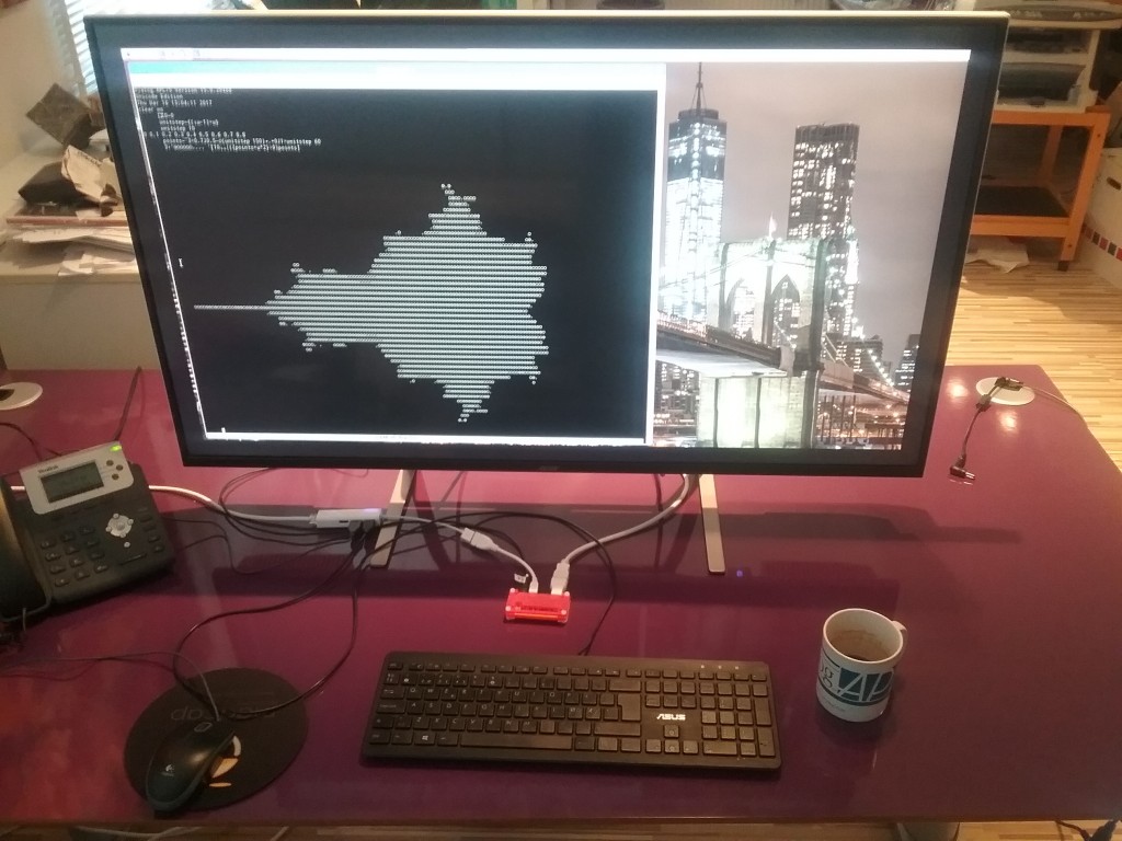
beauty-and-the-beastFinally, the last accessory I ordered for my Raspberry Pi Zero (that’s the little red thing behind my keyboard) has arrived – an Acer 43″ ET430K monitor. The Zero won’t quite drive this monitor at its maximum resolution of 3840×2160 pixels, but as you can see, you get enough real estate to do real graphics with “ASCII Art” (well, Unicode Art, anyway)!

Some readers will recognise the image as the famous Mandelbrot Set, named after the mathematician Benoit Mandelbrot, who studied fractals. According to Wikipedia a fractal is a mathematical set that exhibits a repeating pattern displayed at every scale – they are interesting because they produce patterns that are very similar to things we can see around us – both in living organisms and landscapes – they seem to be part of the fundamental fabric of the universe.

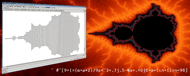
Fractals are are also interesting because they produce images of staggering beauty, as you can see on the pages linked to above and one of our rotating banner pages, where a one-line form of the APL expression which produced the image is embedded:

Website_banner_MbrotW

The colourful images of the Mandelbrot set are produced by looking at a selection of points in the complex plane. For each point c, start with a value of 0 for z, repeat the computation z = c + z², and colour the point according to the number of iterations required before the function becomes “unbounded in value”.

In APL, the function for each iteration can be expressed as {c+⍵*2}, where c is the point and ⍵ (the right argument of the function) is z (initially 0, and subsequently the result of the previous iteration):

      f←{c+⍵*2} ⍝ define the function
      c←1J1     ⍝ c is 1+i (above and to the right of the set)
      (f 0)(f f 0)(f f f 0)(f f f f 0) (f f f f f 0)
1J1 1J3 ¯7J7 1J¯97 ¯9407J¯193

If you are not familiar with complex numbers, those results may look a bit odd. While complex addition just requires adding the real and the imaginary parts independently, the result of multiplication of two complex numbers (a + bi) and (c + di) is defined as (ac-db) + (bc+ad)i. Geometrically, complex multiplication is a combined stretching and rotation operation.

Typing all those f’s gets a bit tedious, fortunately APL has a power operator , a second-order function that can be used to repeatedly apply a function. We can also compute the magnitude of the result number using |:

      (|(f⍣6)0)(|(f⍣7)0)
8.853E7 7.837E15

Let’s take a look at what happens if we choose a point inside the Mandelbrot set:

      c←0.1J0.1
      {|(f⍣⍵)0}¨ 1 2 3 4 5 6 7 8 9 10
0.1414 0.1562 0.1566 0.1552 0.1547 0.1546 0.1546 0.1546 0.1546 0.1546

Above, I used an anonymous function so I could pass the number of iterations in as a parameter, and use the each operator ¨ to generate all the results up to ten iterations. In this case, we can see that the magnitude of the result stabilises, which is why the point 0.1 + 0.1i is considered to be inside the Mandelbrot set.

Points which are just outside the set will require varying numbers of applications of f before the magnitude “explodes”, and if you colour points according to how many iterations are needed and pick interesting areas along the edge of the set, great beauty is revealed.

1200px-GalaxyOfGalaxies

The above image is in the public domain and was created by Jonathan J. Dickau using ChaosPro 3.3 software, which was created by Martin Pfingstl.

Our next task is to create array of points in the complex plane. A helper function unitstep generates values between zero and 1 with a desired number of steps, so I can vary the resolution and size of the image. Using it, I can create two ranges, multiply one of them by i (0J1 in APL) and use an addition table (∘.+) to generate the array:

      ⎕io←0 ⍝ use index origin zero
      unitstep←{(⍳⍵+1)÷⍵}
      unitstep 6
0 0.1667 0.3333 0.5 0.6667 0.8333 1
      c←¯3 × 0.7J0.5 - (0J1×unitstep 6)∘.+unitstep 6
      c
¯2.1J¯1.5 ¯1.6J¯1.5 ¯1.1J¯1.5 ¯0.6J¯1.5 ¯0.1J¯1.5 0.4J¯1.5 0.9J¯1.5
¯2.1J¯1   ¯1.6J¯1   ¯1.1J¯1   ¯0.6J¯1   ¯0.1J¯1   0.4J¯1   0.9J¯1  
¯2.1J¯0.5 ¯1.6J¯0.5 ¯1.1J¯0.5 ¯0.6J¯0.5 ¯0.1J¯0.5 0.4J¯0.5 0.9J¯0.5
¯2.1      ¯1.6      ¯1.1      ¯0.6      ¯0.1      0.4      0.9     
¯2.1J00.5 ¯1.6J00.5 ¯1.1J00.5 ¯0.6J00.5 ¯0.1J00.5 0.4J00.5 0.9J00.5
¯2.1J01   ¯1.6J01   ¯1.1J01   ¯0.6J01   ¯0.1J01   0.4J01   0.9J01  
¯2.1J01.5 ¯1.6J01.5 ¯1.1J01.5 ¯0.6J01.5 ¯0.1J01.5 0.4J01.5 0.9J01.5

The result is subtracted from 0.7J0.5 (0.7 + 0.5i) to get the origin of the complex plane slightly off centre in the middle, and multiplied the whole thing by 3 to get a set of values that brackets the Mandelbrot set.

Note that APL expressions are typically rank and shape invariant, so our function f can be applied to the entire array without changes. Since our goal is only to produce ASCII art, we don’t need to count iterations, we can just compare the magnitude of the result with 9 to decide whether the point has escaped:

      9<|f 0
0 0 0 0 0 0 0
0 0 0 0 0 0 0
0 0 0 0 0 0 0
0 0 0 0 0 0 0
0 0 0 0 0 0 0
0 0 0 0 0 0 0
0 0 0 0 0 0 0
      9<|(f⍣3) 0 ⍝ Apply f 3 times
1 1 1 0 0 0 1
1 0 0 0 0 0 0
0 0 0 0 0 0 0
0 0 0 0 0 0 0
0 0 0 0 0 0 0
1 0 0 0 0 0 0
1 1 1 0 0 0 1

We can see that points around the edge start escaping after 3 iterations. Using an anonymous function again, we can observe more and more points escape, until we recognise the (very low resolution) outline of the Mandelbrot set:


      ]box on
      {((⍕⍵)@(⊂0 0))' #'[9>|(f⍣⍵)0]}¨2↓⍳9
┌───────┬───────┬───────┬───────┬───────┬───────┬───────┐
│2######│3  ### │4      │5      │6      │7      │8      │
│#######│ ######│   ### │    #  │    #  │    #  │    #  │
│#######│#######│ ##### │  #### │  #### │   ### │   ### │
│#######│#######│###### │ ##### │ ##### │ ##### │ ####  │
│#######│#######│ ##### │  #### │  #### │   ### │   ### │
│#######│ ######│   ### │    #  │    #  │    #  │    #  │
│#######│   ### │       │       │       │       │       │
└───────┴───────┴───────┴───────┴───────┴───────┴───────┘

The last example allowed me to sneak in a preview of the new “at” operator coming in Dyalog v16.0. It is a functional merge operator that I am using to insert the formatted right argument (the number of iterations) into position (0 0) of each matrix.

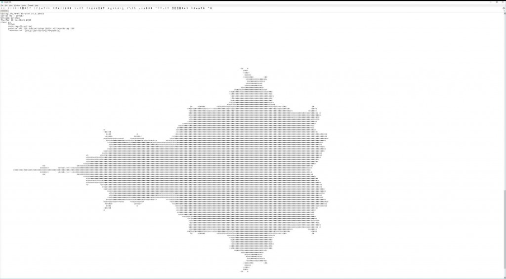
If I use our remote IDE (RIDE) on my Windows machine and connect to the Pi, I can have an APL session on the Pi with 3840×2160 resolution. In this example, I experimented with grey scale “colouring” the result by rounding down and capping the result at 10, and using the character ⍟ (darkest) for 0, ○ for 1-5, × for 6-9, and blank for points that “escaped”, by indexing into an array of ten characters:

      '⍟○○○○○×××× '[10⌊⌊|(f⍣9)c]

Who needs OpenGL?! (click on the image to enlarge)

mandelbrot-ride4

Charting Reaction Times on the Raspberry Pi

Earlier this week I collected some reaction timer data on my Pi using the BBC micro:bit as an input device. I only produced an “ASCII art” chart at the time:

      times←ReactionTimer.Play
      times
251 305 294 415 338 298 294 251 378
      ReactionTimer.AsciiChart times
425| 
400|    * 
375|         *
350+ 
325|     * 
300|  * 
275|   *  ** 
250+ *      * 

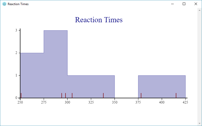
Retro is back in style – but of course I should point out that we can produce “proper” graphics using SharpPlot, a cross-platform graphics package that is included with Dyalog APL on all platforms. I’ve enhanced the ReactionTimer namespace with a function called SPHistogram. If you are using RIDE as the front end to APL on the Pi, this will render output from SharpPlot in a window:

    ReactionTimer.SPHistogram times

Reaction Time Histogram

The original ASCII chart simply plotted the observations in the order that they occurred. Above, the shaded areas show how many observations there were in each bucket (2 between 250ms and 275ms, 3 between 275ms and 300ms, and so on). At the same time, the individual observations can be seen along the X axis as vertical red lines. It is a little unfortunate that, presumably due to some artifact of the timing process, the values 251 and 294 occur twice – and these lines are drawn on top of each other.

The example highlights one of the things that makes SharpPlot a bit special: We have overlaid a histogram showing the frequency of reactions in each bucket, and used a “scatterplot” to where the Y value is always 0, to mark the individual observations along the X axis.

     ∇ SPHistogram times;heading;renderHtml;sp;svg;z 
[1]   heading←'Reaction Times' 
[2]   renderHtml←3500⌶ ⍝ Render HTML in Window 
[3] 
[4]   :If 0=⎕NC'#.SharpPlot' ⋄ #.⎕CY'sharpplot.dws' ⋄ :EndIf
[5] 
[6]   sp←⎕NEW #.SharpPlot(432 250) 
[7]   sp.Heading←heading 
[8] 
[9]   ⍝ Draw histogram 
[10]  sp.ClassInterval←25 
[11]  sp.SetXTickMarks 25 
[12]  sp.HistogramStyle←#.HistogramStyles.SurfaceShading 
[13]  sp.SetFillStyles #.FillStyle.Opacity30 
[14]  sp.DrawHistogram⊂times 
[15] 
[16]  ⍝ Add observations using ScatterPlot 
[17]  sp.SetMarkers #.Marker.UpTick 
[18]  sp.SetPenWidths 1 
[19]  sp.SetMarkerScales 3 
[20]  sp.DrawScatterPlot(times×0)(times) 
[21] 
[22]  ⍝ Render SVG and display in window 
[23]  svg←sp.RenderSvg #.SvgMode.FixedAspect 
[24]  z←heading renderHtml svg 
     ∇ 

Hopefully the code is more or less self-explanatory, but if you’d like to learn more about SharpPlot there is excellent documentation at http://sharpplot.com. The documentation is actually written for C# users, but there is an illustration of how to translate the documentation to APL (and VB) at http://www.sharpplot.com/Languages.htm.

APL Exercises

These exercises are designed to introduce APL to a high school senior adept in mathematics. The entire set of APL Exercises has the following sections:

Introduction
0. Beginnings
1. Utilities
2. Recursion
3. Proofs
4. Rank Operator
5. Index-Of
6. Key Operator
7. Indexing
8. Grade and Sort
9. Power Operator
10. Arithmetic
11. Combinatorial Objects
The Fine Print

Sections 2 and 10 are the most interesting ones and are as follows. The full set is too lengthy (and too boring?) to be included here. Some students may be able to make up their own exercises from the list of topics. As well, it may be useful to know what the “experts” think are important aspects of APL.

2. Recursion

⎕io←0 throughout.

2.0 Factorial

Write a function to compute the factorial function on integer , ⍵≥0.

      fac¨ 5 6 7 8
120 720 5040 40320

      n←1+?20
      (fac n) = n×fac n-1
1
      fac 0
1

2.1 Fibonacci Numbers

Write a function to compute the -th Fibonacci number, ⍵≥0.

      fib¨ 5 6 7 8
5 8 13 21    

      n←2+?20
      (fib n) = (fib n-2) + (fib n-1)
1
      fib 0
0
      fib 1
1

If the function written above is multiply recursive, write a version which is singly recursive (only one occurrence of ). Use cmpx to compare the performance of the two functions on the argument 35.

2.2 Peano Addition

Let and be natural numbers (non-negative integers). Write a function padd to compute ⍺+⍵ without using + itself (or - or × or ÷ …). The only functions allowed are comparison to 0 and the functions pre←{⍵-1} and suc←{⍵+1}.

2.3 Peano Multiplication

Let and be natural numbers (non-negative integers). Write a function ptimes to compute ⍺×⍵ without using × itself (or + or - or ÷ …). The only functions allowed are comparison to 0 and the functions pre←{⍵-1} and suc←{⍵+1} and padd.

2.4 Binomial Coefficients

Write a function to produce the binomal coefficients of order , ⍵≥0.

      bc 0
1
      bc 1
1 1
      bc 2
1 2 1
      bc 3
1 3 3 1
      bc 4
1 4 6 4 1

2.5 Cantor Set

Write a function to compute the Cantor set of order , ⍵≥0.

      Cantor 0
1
      Cantor 1
1 0 1
      Cantor 2
1 0 1 0 0 0 1 0 1
      Cantor 3
1 0 1 0 0 0 1 0 1 0 0 0 0 0 0 0 0 0 1 0 1 0 0 0 1 0 1

The classical version of the Cantor set starts with the interval [0,1] and at each stage removes the middle third from each remaining subinterval:

[0,1] →
[0,1/3] ∪ [2/3,1] →
[0,1/9] ∪ [2/9,1/3] ∪ [2/3,7/9] ∪ [8/9,1] → ….

      {(+⌿÷≢)Cantor ⍵}¨ 3 5⍴⍳15
1         0.666667  0.444444   0.296296   0.197531  
0.131687  0.0877915 0.0585277  0.0390184  0.0260123 
0.0173415 0.011561  0.00770735 0.00513823 0.00342549

      (2÷3)*3 5⍴⍳15
1         0.666667  0.444444   0.296296   0.197531  
0.131687  0.0877915 0.0585277  0.0390184  0.0260123 
0.0173415 0.011561  0.00770735 0.00513823 0.00342549

2.6 Sierpinski Carpet

Write a function to compute the Sierpinski Carpet of order , ⍵≥0.

      SC 0
1
      SC 1
1 1 1
1 0 1
1 1 1
      SC 2
1 1 1 1 1 1 1 1 1
1 0 1 1 0 1 1 0 1
1 1 1 1 1 1 1 1 1
1 1 1 0 0 0 1 1 1
1 0 1 0 0 0 1 0 1
1 1 1 0 0 0 1 1 1
1 1 1 1 1 1 1 1 1
1 0 1 1 0 1 1 0 1
1 1 1 1 1 1 1 1 1

      ' ⌹'[SC 3]
⌹⌹⌹⌹⌹⌹⌹⌹⌹⌹⌹⌹⌹⌹⌹⌹⌹⌹⌹⌹⌹⌹⌹⌹⌹⌹⌹
⌹ ⌹⌹ ⌹⌹ ⌹⌹ ⌹⌹ ⌹⌹ ⌹⌹ ⌹⌹ ⌹⌹ ⌹
⌹⌹⌹⌹⌹⌹⌹⌹⌹⌹⌹⌹⌹⌹⌹⌹⌹⌹⌹⌹⌹⌹⌹⌹⌹⌹⌹
⌹⌹⌹   ⌹⌹⌹⌹⌹⌹   ⌹⌹⌹⌹⌹⌹   ⌹⌹⌹
⌹ ⌹   ⌹ ⌹⌹ ⌹   ⌹ ⌹⌹ ⌹   ⌹ ⌹
⌹⌹⌹   ⌹⌹⌹⌹⌹⌹   ⌹⌹⌹⌹⌹⌹   ⌹⌹⌹
⌹⌹⌹⌹⌹⌹⌹⌹⌹⌹⌹⌹⌹⌹⌹⌹⌹⌹⌹⌹⌹⌹⌹⌹⌹⌹⌹
⌹ ⌹⌹ ⌹⌹ ⌹⌹ ⌹⌹ ⌹⌹ ⌹⌹ ⌹⌹ ⌹⌹ ⌹
⌹⌹⌹⌹⌹⌹⌹⌹⌹⌹⌹⌹⌹⌹⌹⌹⌹⌹⌹⌹⌹⌹⌹⌹⌹⌹⌹
⌹⌹⌹⌹⌹⌹⌹⌹⌹         ⌹⌹⌹⌹⌹⌹⌹⌹⌹
⌹ ⌹⌹ ⌹⌹ ⌹         ⌹ ⌹⌹ ⌹⌹ ⌹
⌹⌹⌹⌹⌹⌹⌹⌹⌹         ⌹⌹⌹⌹⌹⌹⌹⌹⌹
⌹⌹⌹   ⌹⌹⌹         ⌹⌹⌹   ⌹⌹⌹
⌹ ⌹   ⌹ ⌹         ⌹ ⌹   ⌹ ⌹
⌹⌹⌹   ⌹⌹⌹         ⌹⌹⌹   ⌹⌹⌹
⌹⌹⌹⌹⌹⌹⌹⌹⌹         ⌹⌹⌹⌹⌹⌹⌹⌹⌹
⌹ ⌹⌹ ⌹⌹ ⌹         ⌹ ⌹⌹ ⌹⌹ ⌹
⌹⌹⌹⌹⌹⌹⌹⌹⌹         ⌹⌹⌹⌹⌹⌹⌹⌹⌹
⌹⌹⌹⌹⌹⌹⌹⌹⌹⌹⌹⌹⌹⌹⌹⌹⌹⌹⌹⌹⌹⌹⌹⌹⌹⌹⌹
⌹ ⌹⌹ ⌹⌹ ⌹⌹ ⌹⌹ ⌹⌹ ⌹⌹ ⌹⌹ ⌹⌹ ⌹
⌹⌹⌹⌹⌹⌹⌹⌹⌹⌹⌹⌹⌹⌹⌹⌹⌹⌹⌹⌹⌹⌹⌹⌹⌹⌹⌹
⌹⌹⌹   ⌹⌹⌹⌹⌹⌹   ⌹⌹⌹⌹⌹⌹   ⌹⌹⌹
⌹ ⌹   ⌹ ⌹⌹ ⌹   ⌹ ⌹⌹ ⌹   ⌹ ⌹
⌹⌹⌹   ⌹⌹⌹⌹⌹⌹   ⌹⌹⌹⌹⌹⌹   ⌹⌹⌹
⌹⌹⌹⌹⌹⌹⌹⌹⌹⌹⌹⌹⌹⌹⌹⌹⌹⌹⌹⌹⌹⌹⌹⌹⌹⌹⌹
⌹ ⌹⌹ ⌹⌹ ⌹⌹ ⌹⌹ ⌹⌹ ⌹⌹ ⌹⌹ ⌹⌹ ⌹
⌹⌹⌹⌹⌹⌹⌹⌹⌹⌹⌹⌹⌹⌹⌹⌹⌹⌹⌹⌹⌹⌹⌹⌹⌹⌹⌹

3-D analogs of the Cantor set and the Sierpinski carpet are the Sierpinski sponge or the Menger sponge.

2.7 Extended H

Write a function for the extend H algorithm for , ⍵≥0, which embeds the complete binary tree of depth on the plane. In ×H ⍵ there are 2*⍵ leaves, instances of the letter o with exactly one neighbor (or no neighbors for 0=⍵). The root is at the center of the matrix.

      xH¨ ⍳5
┌─┬─────┬─────┬─────────────┬─────────────┐
│o│o-o-o│o   o│o-o-o   o-o-o│o   o   o   o│
│ │     │|   |│  |       |  │|   |   |   |│
│ │     │o-o-o│  o---o---o  │o-o-o   o-o-o│
│ │     │|   |│  |       |  │| | |   | | |│
│ │     │o   o│o-o-o   o-o-o│o | o   o | o│
│ │     │     │             │  |       |  │
│ │     │     │             │  o---o---o  │
│ │     │     │             │  |       |  │
│ │     │     │             │o | o   o | o│
│ │     │     │             │| | |   | | |│
│ │     │     │             │o-o-o   o-o-o│
│ │     │     │             │|   |   |   |│
│ │     │     │             │o   o   o   o│
└─┴─────┴─────┴─────────────┴─────────────┘

Write a function that has the same result as xH but checks the result using the assert utility. For example:

assert←{⍺←'assertion failure' ⋄ 0∊⍵:⍺ ⎕SIGNAL 8 ⋄ shy←0}

xH1←{
  h←xH ⍵
  assert 2=⍴⍴h:
  assert h∊'○ -|':
  assert (¯1+2*1+⍵)=+/'o'=,h:
  ...
  h
}

2.8 Tower of Hanoi

(By André Karwath aka Aka (Own work) [CC BY-SA 2.5 (http://creativecommons.org/licenses/by-sa/2.5)], via Wikimedia Commons)

The Tower of Hanoi problem is to move a set of different-sized disks from one peg to another, moving one disk at a time, using an intermediate peg if necessary. At all times no larger disk may sit on top of a smaller disk.

Write a function Hanoi to solve the problem of moving disks from peg 0 to peg 2. Since it’s always the disk which is at the top of a peg which is moved, the solution can be stated as a 2-column matrix with column 0 indicating the source peg and column 1 the destination peg.

      Hanoi¨ ⍳5
┌───┬───┬───┬───┬───┐
│   │0 2│0 1│0 2│0 1│
│   │   │0 2│0 1│0 2│
│   │   │1 2│2 1│1 2│
│   │   │   │0 2│0 1│
│   │   │   │1 0│2 0│
│   │   │   │1 2│2 1│
│   │   │   │0 2│0 1│
│   │   │   │   │0 2│
│   │   │   │   │1 2│
│   │   │   │   │1 0│
│   │   │   │   │2 0│
│   │   │   │   │1 2│
│   │   │   │   │0 1│
│   │   │   │   │0 2│
│   │   │   │   │1 2│
└───┴───┴───┴───┴───┘

Prove that Hanoi ⍵ has ¯1+2*⍵ rows.

10. Arithmetic

⎕io←0 throughout.

10.0 Primality Testing

Write a function prime ⍵ which is 1 or 0 depending on whether non-negative integer is a prime number. For example:

      prime 1
0
      prime 2
1
      prime 9
0
      prime¨ 10 10⍴⍳100
0 0 1 1 0 1 0 1 0 0
0 1 0 1 0 0 0 1 0 1
0 0 0 1 0 0 0 0 0 1
0 1 0 0 0 0 0 1 0 0
0 1 0 1 0 0 0 1 0 0
0 0 0 1 0 0 0 0 0 1
0 1 0 0 0 0 0 1 0 0
0 1 0 1 0 0 0 0 0 1
0 0 0 1 0 0 0 0 0 1
0 0 0 0 0 0 0 1 0 0

10.1 Primes Less Than n

Write a function primes ⍵ using the sieve method which produces all the primes less than . Use cmpx to compare the speed of primes n and (prime¨⍳n)/⍳n. For example:

      primes 7
2 3 5
      primes 50
2 3 5 7 11 13 17 19 23 29 31 37 41 43 47

      (prime¨⍳50)/⍳50
2 3 5 7 11 13 17 19 23 29 31 37 41 43 47

10.2 Factoring

Write a function factor which produces the prime factorization of , such that ⍵ = ×/factor ⍵ and ∧/ prime¨ factor ⍵ is 1. For example:

      factor 144
2 2 2 2 3 3
      ×/ factor 144
144
      ∧/ prime¨ factor 144
1

      factor 1

      factor 2
2

10.3 pco

Read about the pco function in http://dfns.dyalog.com/n_pco.htm and experiment with it.

      )copy dfns pco

      pco ⍳7
2 3 5 7 11 13 17

      1 pco ⍳10
0 0 1 1 0 1 0 1 0 0

G.H. Hardy states in A Mathematician’s Apology (chapter 14, page 23) that the number of primes less than 1e9 is 50847478. Use pco to check whether this is correct.

10.4 GCD

Write a function ⍺ gcd ⍵ to compute the greatest common divisor of non-negative integers and using the Euclidean algorithm.

Write a function ⍺ egcd ⍵ to compute the GCD of and as coefficients of and , such that (⍺ gcd ⍵) = (⍺,⍵)+.×⍺ egcd ⍵.

      112 gcd 144
16
      112 egcd 144
4 ¯3
      112 144 +.× 112 egcd 144
16

10.5 Ring Extension

Z[√k] is the ring of integers Z extended with √k where k is not a perfect square. The elements of Z[√k] are ordered pairs (a,b) which can be interpreted as a+b×√k (a+b×k*0.5).

Write a d-operator ⍺(⍺⍺ rplus)⍵ which does addition in Z[√⍺⍺].

      3 4 (5 rplus) ¯2 7
1 11

Write a d-operator ⍺(⍺⍺ rtimes)⍵ which does multiplication in Z[√⍺⍺].

      3 4 (5 rtimes) ¯2 7
134 13

Both of the above can be done using integer operations only.

10.6 Repeated Squaring I

Write a function ⍺ pow ⍵ that computes ⍺*⍵ using repeated squaring. is a number and a non-negative integer. Hint: the binary representation of an integer n obtains as 2⊥⍣¯1⊢n.

10.7 Repeated Squaring II

Write a d-operator ⍺(⍺⍺ rpow)⍵ that computes raised to the power using repeated squaring. is in Z[√⍺⍺] and is a non-negative integer.

      ⊃ (5 rtimes)/ 13 ⍴ ⊂ 1 1
2134016 954368

      1 1 (5 rpow) 13
2134016 954368
      1 ¯1 (5 rpow) 13
2134016 ¯954368

The last two expressions are key steps in an O(⍟n) computation of the n-th Fibonacci number using integer operations, using Binet’s formula: