These exercises are designed to introduce APL to a high school senior adept in mathematics. The entire set of APL Exercises has the following sections:
Introduction
0. Beginnings
1. Utilities
2. Recursion
3. Proofs
4. Rank Operator
5. Index-Of |
6. Key Operator
7. Indexing
8. Grade and Sort
9. Power Operator
10. Arithmetic
11. Combinatorial Objects
The Fine Print |
Sections 2 and 10 are the most interesting ones and are as follows. The full set is too lengthy (and too boring?) to be included here. Some students may be able to make up their own exercises from the list of topics. As well, it may be useful to know what the “experts” think are important aspects of APL.
2. Recursion
⎕io←0 throughout.
2.0 Factorial
Write a function to compute the factorial function on integer ⍵, ⍵≥0.
      fac¨ 5 6 7 8
120 720 5040 40320

      n←1+?20
      (fac n) = n×fac n-1
1
      fac 0
1
2.1 Fibonacci Numbers
Write a function to compute the ⍵-th Fibonacci number, ⍵≥0.
      fib¨ 5 6 7 8
5 8 13 21

      n←2+?20
      (fib n) = (fib n-2) + (fib n-1)
1
      fib 0
0
      fib 1
1
If the function written above is multiply recursive, write a version which is singly recursive (only one occurrence of ∇). Use cmpx to compare the performance of the two functions on the argument 35.
2.2 Peano Addition
Let ⍺ and ⍵ be natural numbers (non-negative integers). Write a function padd to compute ⍺+⍵ without using + itself (or - or × or ÷ …). The only functions allowed are comparison to 0 and the functions pre←{⍵-1} and suc←{⍵+1}.
2.3 Peano Multiplication
Let ⍺ and ⍵ be natural numbers (non-negative integers). Write a function ptimes to compute ⍺×⍵ without using × itself (or + or - or ÷ …). The only functions allowed are comparison to 0 and the functions pre←{⍵-1} and suc←{⍵+1} and padd.
2.4 Binomial Coefficients
Write a function to produce the binomal coefficients of order ⍵, ⍵≥0.
      bc 0
1
      bc 1
1 1
      bc 2
1 2 1
      bc 3
1 3 3 1
      bc 4
1 4 6 4 1
2.5 Cantor Set
Write a function to compute the Cantor set of order ⍵, ⍵≥0.
      Cantor 0
1
      Cantor 1
1 0 1
      Cantor 2
1 0 1 0 0 0 1 0 1
      Cantor 3
1 0 1 0 0 0 1 0 1 0 0 0 0 0 0 0 0 0 1 0 1 0 0 0 1 0 1
The classical version of the Cantor set starts with the interval [0,1] and at each stage removes the middle third from each remaining subinterval:
[0,1] →
[0,1/3] ∪ [2/3,1] →
[0,1/9] ∪ [2/9,1/3] ∪ [2/3,7/9] ∪ [8/9,1] → ….

      {(+⌿÷≢)Cantor ⍵}¨ 3 5⍴⍳15
1         0.666667  0.444444   0.296296   0.197531
0.131687  0.0877915 0.0585277  0.0390184  0.0260123
0.0173415 0.011561  0.00770735 0.00513823 0.00342549

      (2÷3)*3 5⍴⍳15
1         0.666667  0.444444   0.296296   0.197531
0.131687  0.0877915 0.0585277  0.0390184  0.0260123
0.0173415 0.011561  0.00770735 0.00513823 0.00342549
2.6 Sierpinski Carpet
Write a function to compute the Sierpinski Carpet of order ⍵, ⍵≥0.
      SC 0
1
      SC 1
1 1 1
1 0 1
1 1 1
      SC 2
1 1 1 1 1 1 1 1 1
1 0 1 1 0 1 1 0 1
1 1 1 1 1 1 1 1 1
1 1 1 0 0 0 1 1 1
1 0 1 0 0 0 1 0 1
1 1 1 0 0 0 1 1 1
1 1 1 1 1 1 1 1 1
1 0 1 1 0 1 1 0 1
1 1 1 1 1 1 1 1 1

      ' ⌹'[SC 3]
⌹⌹⌹⌹⌹⌹⌹⌹⌹⌹⌹⌹⌹⌹⌹⌹⌹⌹⌹⌹⌹⌹⌹⌹⌹⌹⌹
⌹ ⌹⌹ ⌹⌹ ⌹⌹ ⌹⌹ ⌹⌹ ⌹⌹ ⌹⌹ ⌹⌹ ⌹
⌹⌹⌹⌹⌹⌹⌹⌹⌹⌹⌹⌹⌹⌹⌹⌹⌹⌹⌹⌹⌹⌹⌹⌹⌹⌹⌹
⌹⌹⌹   ⌹⌹⌹⌹⌹⌹   ⌹⌹⌹⌹⌹⌹   ⌹⌹⌹
⌹ ⌹   ⌹ ⌹⌹ ⌹   ⌹ ⌹⌹ ⌹   ⌹ ⌹
⌹⌹⌹   ⌹⌹⌹⌹⌹⌹   ⌹⌹⌹⌹⌹⌹   ⌹⌹⌹
⌹⌹⌹⌹⌹⌹⌹⌹⌹⌹⌹⌹⌹⌹⌹⌹⌹⌹⌹⌹⌹⌹⌹⌹⌹⌹⌹
⌹ ⌹⌹ ⌹⌹ ⌹⌹ ⌹⌹ ⌹⌹ ⌹⌹ ⌹⌹ ⌹⌹ ⌹
⌹⌹⌹⌹⌹⌹⌹⌹⌹⌹⌹⌹⌹⌹⌹⌹⌹⌹⌹⌹⌹⌹⌹⌹⌹⌹⌹
⌹⌹⌹⌹⌹⌹⌹⌹⌹         ⌹⌹⌹⌹⌹⌹⌹⌹⌹
⌹ ⌹⌹ ⌹⌹ ⌹         ⌹ ⌹⌹ ⌹⌹ ⌹
⌹⌹⌹⌹⌹⌹⌹⌹⌹         ⌹⌹⌹⌹⌹⌹⌹⌹⌹
⌹⌹⌹   ⌹⌹⌹         ⌹⌹⌹   ⌹⌹⌹
⌹ ⌹   ⌹ ⌹         ⌹ ⌹   ⌹ ⌹
⌹⌹⌹   ⌹⌹⌹         ⌹⌹⌹   ⌹⌹⌹
⌹⌹⌹⌹⌹⌹⌹⌹⌹         ⌹⌹⌹⌹⌹⌹⌹⌹⌹
⌹ ⌹⌹ ⌹⌹ ⌹         ⌹ ⌹⌹ ⌹⌹ ⌹
⌹⌹⌹⌹⌹⌹⌹⌹⌹         ⌹⌹⌹⌹⌹⌹⌹⌹⌹
⌹⌹⌹⌹⌹⌹⌹⌹⌹⌹⌹⌹⌹⌹⌹⌹⌹⌹⌹⌹⌹⌹⌹⌹⌹⌹⌹
⌹ ⌹⌹ ⌹⌹ ⌹⌹ ⌹⌹ ⌹⌹ ⌹⌹ ⌹⌹ ⌹⌹ ⌹
⌹⌹⌹⌹⌹⌹⌹⌹⌹⌹⌹⌹⌹⌹⌹⌹⌹⌹⌹⌹⌹⌹⌹⌹⌹⌹⌹
⌹⌹⌹   ⌹⌹⌹⌹⌹⌹   ⌹⌹⌹⌹⌹⌹   ⌹⌹⌹
⌹ ⌹   ⌹ ⌹⌹ ⌹   ⌹ ⌹⌹ ⌹   ⌹ ⌹
⌹⌹⌹   ⌹⌹⌹⌹⌹⌹   ⌹⌹⌹⌹⌹⌹   ⌹⌹⌹
⌹⌹⌹⌹⌹⌹⌹⌹⌹⌹⌹⌹⌹⌹⌹⌹⌹⌹⌹⌹⌹⌹⌹⌹⌹⌹⌹
⌹ ⌹⌹ ⌹⌹ ⌹⌹ ⌹⌹ ⌹⌹ ⌹⌹ ⌹⌹ ⌹⌹ ⌹
⌹⌹⌹⌹⌹⌹⌹⌹⌹⌹⌹⌹⌹⌹⌹⌹⌹⌹⌹⌹⌹⌹⌹⌹⌹⌹⌹
3-D analogs of the Cantor set and the Sierpinski carpet are the Sierpinski sponge or the Menger sponge.
2.7 Extended H
Write a function for the extend H algorithm for ⍵, ⍵≥0, which embeds the complete binary tree of depth ⍵ on the plane. In ×H ⍵ there are 2*⍵ leaves, instances of the letter o with exactly one neighbor (or no neighbors for 0=⍵). The root is at the center of the matrix.
      xH¨ ⍳5
┌─┬─────┬─────┬─────────────┬─────────────┐
│o│o-o-o│o   o│o-o-o   o-o-o│o   o   o   o│
│ │     │|   |│  |       |  │|   |   |   |│
│ │     │o-o-o│  o---o---o  │o-o-o   o-o-o│
│ │     │|   |│  |       |  │| | |   | | |│
│ │     │o   o│o-o-o   o-o-o│o | o   o | o│
│ │     │     │             │  |       |  │
│ │     │     │             │  o---o---o  │
│ │     │     │             │  |       |  │
│ │     │     │             │o | o   o | o│
│ │     │     │             │| | |   | | |│
│ │     │     │             │o-o-o   o-o-o│
│ │     │     │             │|   |   |   |│
│ │     │     │             │o   o   o   o│
└─┴─────┴─────┴─────────────┴─────────────┘
Write a function that has the same result as xH but checks the result using the assert utility. For example:
assert←{⍺←'assertion failure' ⋄ 0∊⍵:⍺ ⎕SIGNAL 8 ⋄ shy←0}

xH1←{
  h←xH ⍵
  assert 2=⍴⍴h:
  assert h∊'○ -|':
  assert (¯1+2*1+⍵)=+/'o'=,h:
  ...
  h
}
2.8 Tower of Hanoi
(By André Karwath aka Aka (Own work) [CC BY-SA 2.5 (http://creativecommons.org/licenses/by-sa/2.5)], via Wikimedia Commons)
The Tower of Hanoi problem is to move a set of ⍵ different-sized disks from one peg to another, moving one disk at a time, using an intermediate peg if necessary. At all times no larger disk may sit on top of a smaller disk.
Write a function Hanoi ⍵ to solve the problem of moving ⍵ disks from peg 0 to peg 2. Since it’s always the disk which is at the top of a peg which is moved, the solution can be stated as a 2-column matrix with column 0 indicating the source peg and column 1 the destination peg.
      Hanoi¨ ⍳5
┌───┬───┬───┬───┬───┐
│   │0 2│0 1│0 2│0 1│
│   │   │0 2│0 1│0 2│
│   │   │1 2│2 1│1 2│
│   │   │   │0 2│0 1│
│   │   │   │1 0│2 0│
│   │   │   │1 2│2 1│
│   │   │   │0 2│0 1│
│   │   │   │   │0 2│
│   │   │   │   │1 2│
│   │   │   │   │1 0│
│   │   │   │   │2 0│
│   │   │   │   │1 2│
│   │   │   │   │0 1│
│   │   │   │   │0 2│
│   │   │   │   │1 2│
└───┴───┴───┴───┴───┘
Prove that Hanoi ⍵ has ¯1+2*⍵ rows.
10. Arithmetic
⎕io←0 throughout.
10.0 Primality Testing
Write a function prime ⍵ which is 1 or 0 depending on whether non-negative integer ⍵ is a prime number. For example:
      prime 1
0
      prime 2
1
      prime 9
0
      prime¨ 10 10⍴⍳100
0 0 1 1 0 1 0 1 0 0
0 1 0 1 0 0 0 1 0 1
0 0 0 1 0 0 0 0 0 1
0 1 0 0 0 0 0 1 0 0
0 1 0 1 0 0 0 1 0 0
0 0 0 1 0 0 0 0 0 1
0 1 0 0 0 0 0 1 0 0
0 1 0 1 0 0 0 0 0 1
0 0 0 1 0 0 0 0 0 1
0 0 0 0 0 0 0 1 0 0
10.1 Primes Less Than n
Write a function primes ⍵ using the sieve method which produces all the primes less than ⍵. Use cmpx to compare the speed of primes n and (prime¨⍳n)/⍳n. For example:
      primes 7
2 3 5
      primes 50
2 3 5 7 11 13 17 19 23 29 31 37 41 43 47

      (prime¨⍳50)/⍳50
2 3 5 7 11 13 17 19 23 29 31 37 41 43 47
10.2 Factoring
Write a function factor ⍵ which produces the prime factorization of ⍵, such that ⍵ = ×/factor ⍵ and ∧/ prime¨ factor ⍵ is 1. For example:
      factor 144
2 2 2 2 3 3
      ×/ factor 144
144
      ∧/ prime¨ factor 144
1

      factor 1

      factor 2
2
10.3 pco
Read about the pco function in http://dfns.dyalog.com/n_pco.htm and experiment with it.
      )copy dfns pco

      pco ⍳7
2 3 5 7 11 13 17

      1 pco ⍳10
0 0 1 1 0 1 0 1 0 0
G.H. Hardy states in A Mathematician’s Apology (chapter 14, page 23) that the number of primes less than 1e9 is 50847478. Use pco to check whether this is correct.
10.4 GCD
Write a function ⍺ gcd ⍵ to compute the greatest common divisor of non-negative integers ⍺ and ⍵ using the Euclidean algorithm.
Write a function ⍺ egcd ⍵ to compute the GCD of ⍺ and ⍵ as coefficients of ⍺ and ⍵, such that (⍺ gcd ⍵) = (⍺,⍵)+.×⍺ egcd ⍵.
      112 gcd 144
16
      112 egcd 144
4 ¯3
      112 144 +.× 112 egcd 144
16
10.5 Ring Extension
Z[√k] is the ring of integers Z extended with √k where k is not a perfect square. The elements of Z[√k] are ordered pairs (a,b) which can be interpreted as a+b×√k (a+b×k*0.5).
Write a d-operator ⍺(⍺⍺ rplus)⍵ which does addition in Z[√⍺⍺].
      3 4 (5 rplus) ¯2 7
1 11
Write a d-operator ⍺(⍺⍺ rtimes)⍵ which does multiplication in Z[√⍺⍺].
      3 4 (5 rtimes) ¯2 7
134 13
Both of the above can be done using integer operations only.
10.6 Repeated Squaring I
Write a function ⍺ pow ⍵ that computes ⍺*⍵ using repeated squaring. ⍺ is a number and ⍵ a non-negative integer. Hint: the binary representation of an integer n obtains as 2⊥⍣¯1⊢n.
10.7 Repeated Squaring II
Write a d-operator ⍺(⍺⍺ rpow)⍵ that computes ⍺ raised to the power ⍵ using repeated squaring. ⍺ is in Z[√⍺⍺] and ⍵ is a non-negative integer.
      ⊃ (5 rtimes)/ 13 ⍴ ⊂ 1 1
2134016 954368

      1 1 (5 rpow) 13
2134016 954368
      1 ¯1 (5 rpow) 13
2134016 ¯954368
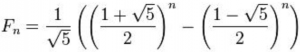
The last two expressions are key steps in an O(⍟n) computation of the n-th Fibonacci number using integer operations, using Binet’s formula:


 Follow