This post might be more difficult than our usual fare. You won’t find any interesting APL coding insights here—instead we’ll be focused on the tricky topic of floating-point error analysis. If that’s not your thing, feel free to skip this one! Although if you plan to use tolerated comparison in a real application, you really do need to know this stuff.

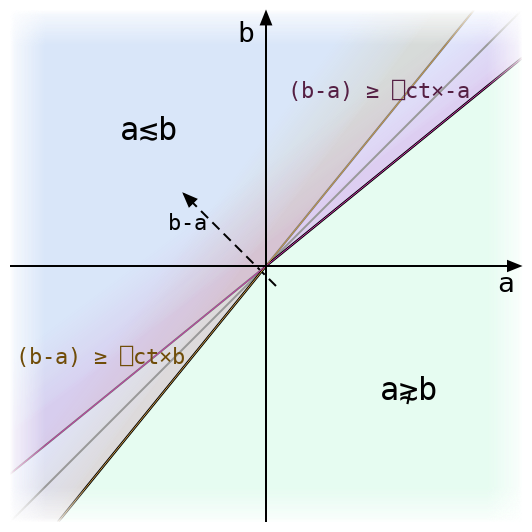
In Tolerated Comparison, Part 1, I discussed the structure of tolerant inequality with one argument fixed, and showed that

• For any real number B, there’s another number b so that a number is tolerantly less than or equal to B if and only if it is intolerantly less than or equal to b.
• This number is equal to B÷1-⎕CT when B<0, and B×1-⎕CT otherwise.

But these results were proven only for mathematical real numbers, which have many properties among which is the complete inability to be implemented in a silicon chip. To actually apply the technique in Dyalog APL, we must know that it works for IEEE floats like Dyalog uses (we have not implemented tolerated comparison for the decimal floating point numbers used when ⎕FR is 1287, and there are serious concerns regarding precision which might make it impossible to tolerate values efficiently).

Why should we care if a tolerated value is off by one or a few units in the last place? It’s certainly unlikely to cause widespread chaos. But we think programmers should be able to expect, for instance, that after setting i←v⍳x it is always safe to assume that v[i]=x. A language that behaves otherwise can easily cause “impossible” bugs in programs that are provably correct according to Dyalog’s specification. And finding a value that lies just on the boundary of equality with x is not as obscure an issue as it may appear. With the default value ⎕CT←1E¯14, there are at most about 180 numbers which are tolerantly equal to a typical floating-point number x. So it’s not much of a stretch to think that a program which handles a lot of similar values will eventually run into a problem with an inaccurate version of tolerated equality. And this is a really scary problem to debug—even the slightest difference in the values used would make it disappear, frustrating any efforts to track down the cause. We’ve dealt with tolerant comparison issues in the past and this kind of problem is certainly not something we want to stumble on in the future.

On to floating-point numbers. I’m afraid this is not a primer on the subject, although I can point any interested readers to the excellent What Every Computer Scientist Should Know About Floating-Point Arithmetic. In brief, Dyalog’s floating-point numbers use 64 bits to represent a particular set of real numbers chosen to cover many orders of magnitude and to satisfy some nice mathematical properties. We need to know only a surprisingly small number of things about these numbers, though—see the short list below. Here we consider only normal numbers, and not denormal numbers, which appear at extremely small magnitudes. The important result of this post is still valid for denormal numbers, which have higher tolerance for error than normal numbers, but we will not demonstrate this detail here.

Definitions: In the discussion below, q is used as a short name for the value ⎕CT. Unless stated otherwise, formulas below are to be interpreted not as floating-point calculations but as mathematical expressions—there is no rounding and all comparisons in formulas are intolerant. Evaluation order follows APL except that = is used as in mathematics: it has lower precedence and can be used multiple times in chains to show that many values are all equal to each other. The word “error” indicates absolute error, that is, the absolute distance of a computed value from some desired value. The value ulp (from “Unit in the Last Place”) is used to indicate what some might denote ULP(1), the distance from 1 to the next higher floating point number. It is equal to 2*¯52, and it is an upper bound on the error between two adjacent normal floating-point numbers divided by the smaller of their magnitudes.

We will require the following facts about floating point numbers:

1. Two adjacent (normal, nonzero) floating-point numbers a and b differ by at least 0.5×(|a)×ulp and at most (|a)×ulp.
2. Consequently, the error introduced by exact rounding in a computation whose exact result is x is at most (|x)×0.5×ulp. The operations +-×÷ are all exactly rounded.
3. Sterbenz’s lemma: If x and y are two floating-point numbers with x≤2×y and y≤2×x, then the difference x-y is exactly equal to a floating-point number. Theorem 11 in the link above is closely related, and its proof indicates how one would prove this fact.
4. Given a floating-point number, the next lower or next higher number can be efficiently computed (in fact, provided the initial number is nonzero, their binary representations differ from that number by exactly 1 when considered as 64-bit integers).

We’ll need one other fact, which Dyalog APL guarantees (other APLs might not). The maximum value of ⎕CT is 2*¯32, chosen so that two 32-bit integers can’t be tolerantly equal to each other. Otherwise, integers couldn’t be compared using the typical CPU instructions, which would be a huge performance problem. The value of ulp is 2*¯52 for IEEE doubles, so ⎕CT*2 is at most ulp÷2*12. The proof below holds for ⎕CT*2 as high as ulp÷9, but not for ⎕CT*2 higher than ulp÷8.

Our task

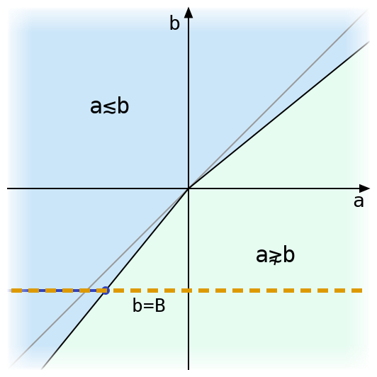
In the following discussion, we will primarily consider the case B>0. We want to define a function tolerateLE which, given B, returns the greatest floating-point value tolerantly less than or equal to B, and to show that every value smaller than tolerateLE B is also tolerantly less than or equal to B. The last post analysed this situation on real (not floating-point) numbers, and showed that in that case tolerateLE B is equal to B÷1-q.

The case B<0 is substantially simpler to analyse, because the formula B×1-q for this case is more tractable. This case is not described fully but can be handled using the same techniques. Also not included is the case B=0. tolerateLE 0 is zero, since comparison with zero is already intolerant.

Error analysis: B÷1-q

(This section isn’t necessary for our proof. But it’s useful to see why the obvious formula isn’t good enough, and serves as a nice warmup before the more difficult computations later.)

When we compute B÷1-q on a computer, how does that differ from the result of computing B÷1-q using the mathematician’s technique of not actually computing it? There are two operations here, and each is subject to floating-point rounding afterwards. To compute the final error we must use an alternating procedure: for each operation, first find the greatest error that could happen if the operation was computed exactly, based on the error in its arguments. Then add another error term for rounding, which is based on the size of the operation’s result.

It’s helpful to know first how inverting a number close to 1 affects its error. Suppose x is such a number, and it has a maximum error x×r. We’ll get the largest possible error by comparing y÷x×1-r to the exact value y÷x (you can verify this by re-doing the calculation below using 1+r instead). The error is

err = | (y÷x) - y÷x×1-r
    = (y÷x) × | 1 - ÷1-r
    = (y÷x) × | r÷1-r

Assuming r<0.5, which will be wildly conservative for our uses, we know that (1-r)>0.5 and hence (÷1-r)<2. So if the absolute error in x is at most x×r, then the absolute error in y÷x (assuming y is exact, and before any rounding) is at most:

err < (y÷x) × 2×r

Now we can figure out the error when evaluating B÷1-q. At each step the rounding error is at most 0.5×ulp times the current value.

⍝computation     error before rounding     error after rounding
1-q              0                         (1-q)×0.5×ulp
B÷1-q            (B÷1-q) × 2×0.5×ulp       (B÷1-q)×1.5×ulp

The actual upper bound on error has a coefficient substantially less than 1.5, since the error estimate for B÷1-q was very conservative. But the important thing is that it’s definitely greater than 1. The value we compute could be one of the two closest to B÷1-q, but it could also be further out. Obviously we can’t guarantee this is the exact value that tolerateLE B should return. But what kind of bounds can we set on that value, anyway?

Evaluating tolerant inequality

The last post showed that, when B>0, a value a is tolerantly less than or equal to B if and only if it is exactly less than or equal to B÷1-q. But that was based on perfectly accurate real numbers. What actually happens around this value for IEEE floats? Let’s say B is some positive floating-point number and at is the exact value of B÷1-q (which might not be a floating-point number). Then suppose a is another floating-point number, and define e (another possibly-non-floating-point number) so that a = at+e. What is the result of evaluating the tolerant less-than formula below?

(a-B) ≤ q × 0⌈a⌈-B

The left-hand side turns out to be very easy to analyse due to Sterbenz’s lemma, which states that if x and y are two floating-point numbers with x≤2×y and y≤2×x, then the difference x-y is exactly equal to a floating-point number, meaning that it will not be rounded at all when it is computed. It’s easy to show that if a>2×B then a is tolerantly greater than B, and that if B>2×a then a is tolerantly less than or equal to B. So in the interesting case, where a is close to B, we know that the following chain of equalities holds exactly:

a-B = e + at-B
    = e + (B÷1-q)-B
    = e + B×(÷1-q)-1
    = e + B×q÷1-q

Now what about the right-hand side? Because B>0 and (by our simplifying assumption in the previous paragraph) a≥B÷2, a is the largest of the three numbers in 0⌈a⌈-B. Floating-point maximum is always exact (since it’s equal to one of its arguments), so the right-hand side simplifies to q×a. This expression does end up rounding. Its value before rounding can be expressed in terms of a-B and e:

q×a = (q×at) + q×e
    = (B×q÷1-q) + q×e
    = (e + B×q÷1-q) - (e - q×e)
    = (a-B) - e×1-q

It’s very helpful here to know that a-B is exactly a floating-point number! q×a will round to a value that is smaller than a-B (thus making the tolerant inequality a≤B come out false) when it is closer to the next-smallest floating-point number than to a-B (if it is halfway between, it could round either way depending on the last bit of a-B). This happens as long as e×1-q is larger than half the distance to that predecessor. The floating-point format guarantees that, as long as a-B is a normal number, this distance is between 0.25×ulp×a-B and 0.5×ulp×a-B, where ulp is the difference between 1 and the next floating-point number. Consequently, if e is less than 0.25×ulp×a-B, we are sure that a will be found tolerantly less than or equal to B, and if e is greater than 0.5×ulp×a-B, it won’t be. If it falls in that range, we can’t be sure.

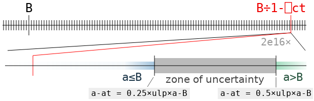
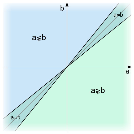
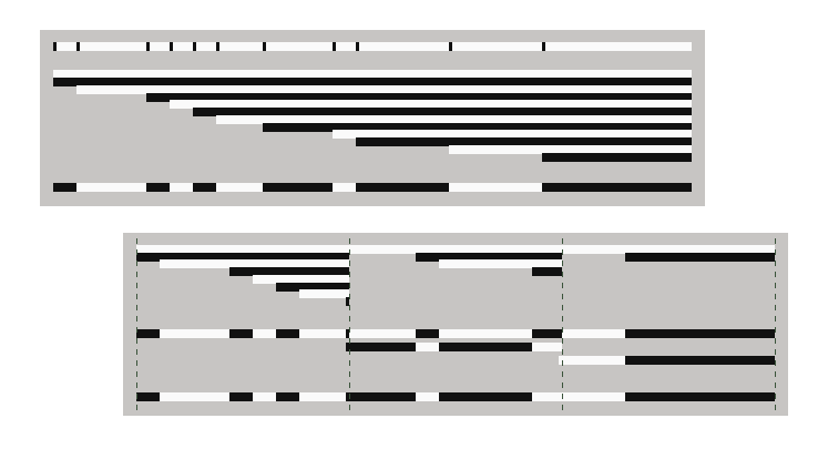
The zone of uncertainty for the value B←2*÷5 is illustrated above. It contains all the values of a for which we can’t say for sure whether a is tolerantly less than or equal to B, or greater, without actually doing the computation and rounding (that is, the result will depend on specifics of the floating-point format and not just ulp). It’s very small! It will almost never contain an actual floating point value (one of the black ticks), but it could.

If there isn’t a floating point number in the zone of uncertainty, then tolerateLE B has to be the first floating point number to its left. But if there is one, say c, then the value depends on whether c is tolerantly less than or equal to B: if it is, then c = tolerateLE B. If not, then that obviously can’t be the case, and tolerateLE B is again the nearest floating point value to the left of the zone of uncertainty.

Error analysis: B+q×B

How can we compute B÷1-q more accurately than our first try? One good way of working with the expression ÷1-x when x is between 0 and 1 is to use its well-known expansion as in infinite polynomial. A mathematically-inclined APLer (who prefers ⎕IO←0) might write

(÷1-x) = +/x*⍳∞

where the right-hand side represents the infinite series 1+x+x²+x³+…. One fact that seems more obvious when thinking about the series than about the reciprocal is that, defining z←÷1-x, we know z = 1+x×z. So similarly,

(B÷1-q) = B+q×B÷1-q

But it turns out to be much easier than that! The difference between 1 and ÷1-q is fairly close to q. So if we replace ÷1-q by 1, then we end up off by about B×q×q. Knowing that q*2 is much smaller than ulp, we see that this difference is miniscule compared to B. So why don’t we try the expression B+q×B?

The error in using B instead of B÷1-q is

(|B - B÷1-q) = |B × 1-÷1-q
             = |B × ((1-q)-1)÷1-q
             = B × q÷1-q

Multiplying by q, the absolute error of q×B is q×B × q÷1-q, which, knowing that (÷1-q)<2, is less than B × 2×q*2, and consequently less than, say, B×0.05×ulp.

⍝computation   relative to    err before rounding   err after rounding
q×B            q×B÷1-q        B×0.05×ulp            B×(0.05+q)×ulp
B+q×B          B÷1-q          B×0.06×ulp

That’s pretty close: the unrounded error is substantially less than the error that will be introduced by the final rounding (about B×0.5×ulp). Chances are, it’s the closest floating point number to B÷1-q. But it could wind up on either side of that value, so we will need to perform a final adjustment to obtain tolerateLE B.

Note that the new formula B+q×B is very similar to the formula B×1-q which is used when B is negative. In fact, calculating the latter value with the expression B+q×-B will also have a very low error. That means we can use B+q×|B for both cases! However, we will still need to distinguish between them when testing whether the value that we get is actually tolerantly less than or equal to B.

Polishing up

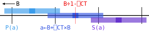
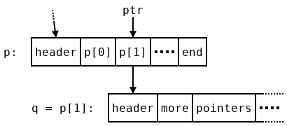
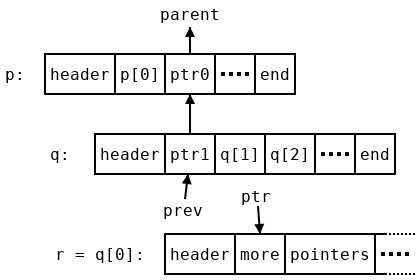
After we calculate a←B+q×B, we still don’t know which way a≤B will go. There’s just too much error to make sure it falls on one side or the other of the critical band. But we do know about the numbers just next to it: a value adjacent to a must be separated from the unrounded value of B+q×B by at least 0.25×B×(1+q)×ulp, or else we would have rounded a towards it. That unrounded value differs from the true value B÷1-q by only 0.06×B×ulp at most, so we know that these neighbors are at least ((0.25×1+q)-0.06)×B×ulp or (rounding down some) 0.15×B×ulp from at. But that’s way outside of the zone of uncertainty, which goes out only to 0.5×ulp×a-B, since a-B is somewhere around q×B.

So we know that the predecessor to a must be tolerantly less than or equal to B, and its sucessor must not be. That leaves us with only two possibilities: either a is tolerantly less than or equal to B, in which case it is the largest floating-point number with this property, or it isn’t, in which case its predecessor is that number. In the diagram above, we can see that the range for a is a little bigger than the gap between ticks, but it’s small enough that the ranges for its predecessor P(a) and successor S(a) don’t overlap with B÷1-⎕CT or the invisibly small zone of uncertainty to its right. In this case a rounds left, so a = tolerateLE B, but if it rounded right, then we would have (P(a)) = tolerateLE B.

So that’s the algorithm! Just compute B+q×|B, and compare to see if it is tolerantly less than or equal to B. If it is, return it, and otherwise, return its predecessor, the next floating point number in the direction of negative infinity. We also add checks to the Dyalog interpreter’s debug mode to make sure the number returned is actually tolerantly less than or equal to B, and that the next larger one isn’t.

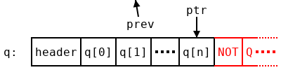
APL model

The following code implements the ideas above in APL. Note that it can give a domain error for numbers near the edges of the floating-point range; Dyalog’s internal C implementation has checks to handle these cases properly. adjFP does some messy work with the binary representation of a floating-point value in order to add or subtract one from the integer it represents. Once that’s out of the way, tolerated inequalities are very simple!

⍝ Return the next smaller floating-point number if ⍺ is ¯1, or the
⍝ next larger if ⍺ is 1 (default).
⍝ Not valid if ⍵=0.
adjFP ← {
  ⍺←1 ⋄ x←(⍺≥0)≠⍵≥0
  bo←,∘⌽(8 8∘⍴)⍣(~⊃83 ⎕DR 256) ⍝ Order bits little-endian (self-inverse)
  ⊃645⎕DR bo (⊢≠¯1↓1,(∧\x≠⊢)) bo 11⎕DR ⊃0 645⎕DR ⍵
}

⍝ Tolerate the right-hand side of an inequality.
⍝ tolerateLE increases its argument while tolerantGE decreases it.
⍝ tolerantEQ returns the smallest and largest values equal to its argument.
tolerateLE ← { ¯1 adjFP⍣(t>⍵)⊢ t←⍵+⎕ct×|⍵ }
tolerateGE ← -∘tolerateLE∘-
tolerateEQ ← tolerateGE , tolerateLE

We can see below that tolerateEQ returns values which are tolerantly equal to the original argument, but which are adjacent to other values that aren’t.

      (⊢=tolerateEQ) 2*÷5
1 1
      (⊢=¯1 1 adjFP¨ tolerateEQ) 2*÷5
0 0

Of course, using tolerateEQ followed by intolerant comparison won’t speed anything up in version 17.0: that’s already been done!

Follow

Warning: The formula for “tolerated” comparison in this post is not correct for actual floating-point numbers. Do not use it! The follow-up post discusses how to compute the required value precisely in the presence of floating-point error.

Tolerant comparison is an important feature in making APL usable in the real world. But it’s also a lot slower than exact comparison. We think this tradeoff is well worth it (and of course, if you don’t want to make it, just set ⎕CT←0). But once in a while we can completely get rid of the slowdown! Added in Dyalog 17.0, along with vectorised comparison code so fast you might not even notice this change, is a cool technique that I call “tolerated comparison”. It works by turning a tolerant comparison with one argument fixed into an intolerant comparison by adjusting that fixed argument. So if you’re comparing one floating-point number to many of them, your code will run 30-40% faster than it would without this improvement.

Why tolerance?

Let’s take a trip to a slightly different APL.

      ⎕CT←0

A world in which tolerant comparison hasn’t been invented. Two things are equal when they’re the same.

      0.1 = 0.3-0.2
0
      {(0.1×⍵) = ⍵÷10} ⍳8
1 1 0 1 1 0 0 1

Okay, that’s a scary place. What happened?

The floating-point format can’t possibly represent every real number. Instead, there’s a carefully chosen set containing just shy of 2*64 numbers which can be expressed. For other numbers, we pick the closest available floating-point number. Usually this is a pretty accurate approximation. But once we perform arithmetic with a few of these values, we might go from “closest possible approximation” to “second-closest approximation” or even further away. The differences are still tiny, but when the same value—mathematically speaking—is computed in two different ways the results might be different numbers. Just barely different, but in a world without tolerant comparison that means they won’t be equal any more.

Tolerant comparison is an attempt to fix this. It’s not perfect, but it’s better in a lot of real-world situations. It makes = a useful function. The rule is that two values are equal when their difference is at most ⎕CT times the larger of their magnitudes. This is often called a “relative epsilon comparison” outside of the APL world.

Notation: To avoid confusion in the following text, I have used the APL symbols <≤=≥>≠ for intolerant comparisons, and the non-APL symbols ⋦≲≂≳⋧≉ to refer to APL’s tolerant comparisons which depend on ⎕CT. Watch out for a few quirks due to the scarcity of symbols to use: the actual APL primitives are denoted by non-APL characters, and the simpler symbol < “less-than” corresponds to the more complicated ⋦ “less-than and not approximately equal to”.

Tolerant comparisons

The famous formula for tolerant equality a≂b in terms of intolerant inequality (introduced here) is

(|a-b) ≤ ⎕CT×(|a)⌈(|b)

This allows for a little variation in the arguments, provided that neither one is zero. And it has some other nice properties, assuming ⎕CT≤1:

• It’s reflexive: a≂a for any number a.
• It’s symmetric in a and b: reversing them makes no difference in the result. This is because ⌈ and (|-) are symmetric functions.
• It scales linearly: multiplying both a and b by the same nonzero value (even a negative number) does not change the result.
• It’s convex in each variable: if a≂b and a≂d for some a, and c is between b and d, then a≂c.

In fact, tolerant equality as in APL is the only solution (or family of solutions, taking the ⎕CT parameter into account) to those constraints, other than the trivial one in which any two numbers are equal.

The above figure illustrates tolerant comparison of two real numbers. They are exactly equal only on the grey diagonal line, and tolerantly equal within the narrow strip around it. The diagram uses a much larger value for ⎕CT than Dyalog’s default of 1e¯14, or even its maximum allowed value of 2*¯32, either of which would make that strip invisible.

One way to define tolerant inequalities in terms of tolerant equality is to define, for instance, (a≲b) ≡ (a<b)∨(a≂b) using intolerant less-than and tolerant equality. But we’ll find it more useful to define ≲ and ≳ directly in terms of intolerant comparisons as with ≂. The formula for ≲ is:

(a-b) ≤ ⎕CT × 0⌈a⌈-b

and for ≳ we can use either (a≳b) ≡ (b≲a) or (a≳b) ≡ (-a)≲(-b) to obtain

(b-a) ≤ ⎕CT × 0⌈b⌈-a

or, negating both sides and swapping the inequality,

(a-b) ≥ ⎕CT × 0⌊a⌊-b

The 0⌈ term isn’t strictly necessary (as we’ll show later), but it helps avoid some confusion when a and b have different signs. Sometimes it’s used to speed up comparison by checking if a≤b intolerantly before performing any multiplication—if it is, the multiplication isn’t needed.

Above we can see how the equation for tolerant ≲ splits into two symmetrical half-formulas, each of which is just a little off from the exact inequality a≤b. The tolerant inequality accepts either of these conditions.

The region of tolerant equality is now the intersection of the regions for tolerant ≲ and ≳. That is:

(a≂b) ≡ (a≲b)∧(a≳b)

We’ll find this decomposition handy later on since tolerant inequalities are so much easier to work with.

Tolerating an inequality

What happens if we fix one side of the inequality? Here’s a diagram for a≲b with a dashed line drawn where b is equal to some fixed B and a varies.

There’s only one place where the black line bounding the region where a≲b intersects the line b=B. The value of a at this intersection has an interesting property: when a is (exactly) less than or equal to that value, then it is tolerantly less than or equal to B. If we want to compare B to many other floating-point values, and we know the a coordinate of the intersection above, then we can skip all of the tolerant comparison arithmetic and just use exact comparison with that value!

Once we have a way to do this for ≲ all other inequalities will follow, since (a≳B) ≡ (-a)≲(-B) and (a⋧B) ≡ ~(a≲B).

Maybe you can figure out the value from the graphs above. But it’s also easy to find the value (and prove it works!) using a fact about the maximum function: for real numbers x, y, and z, x≤y⌈z is the same as (x≤y) ∨ (x≤z). One of the advantages of treating inequalities as functions like any other is that formulas like these are easy to manipulate. Here we go:

Start with the formula for tolerant inequality, writing q in place of ⎕CT.

(a-B) ≤ q × 0⌈a⌈-B

Distributing q× over ⌈, we have

(a-B) ≤ 0 ⌈ (q×a) ⌈ (-q×B)

and using (x≤y⌈z) ≡ ((x≤y) ∨ (x≤z)) twice (just like in the previous step, this can be thought of as distributing x≤ over three arguments of an associative function all at once), we can expand this formula to

((a-B) ≤ 0) ∨ ((a-B) ≤ q×a) ∨ ((a-B) ≤ -q×B)

which simplifies to

(a ≤ B) ∨ ((a×1-q) ≤ B) ∨ (a ≤ B×1-q)

or (here we need q<1, so that 1-q is positive; otherwise we’d have to reverse the middle inequality)

(a ≤ B) ∨ (a ≤ B÷1-q) ∨ (a ≤ B×1-q)

Recombining, we get

a  ≤  B ⌈ (B÷1-q) ⌈ (B×1-q)

So that’s our formula: now the tolerant equality is an intolerant equality, where the right side depends only on B!

Reading the signs

So we have a formula for a “tolerated” value b = B ⌈ (B÷1-q) ⌈ (B×1-q). When do the different possible maxima come into play?

• If B=0, then everything on the right is zero, and b=0.
• If B>0, then B×1-q is smaller than B, since q>0. But that means ÷1-q is larger than 1, and B÷1-q is larger than B. So b=B÷1-q.
• If B<0, then the all the inequalities that we got with B>0 are reversed. This means b=B×1-q.

Note that none of these cases depend on the branch b=B, even though the first one touches it. That means the definition of tolerant inequality would be the same even if we remove that branch. By working backwards through the above derivation we find that the initial 0⌈ has no effect, and we can remove it from the definition.

Equality

Tolerant equality obviously can’t be reduced to intolerant equality, since many values can be tolerantly equal to a number but only one is intolerantly equal to it. But recalling that (a≂b) ≡ (a≲b)∧(a≳b), we can express it as two intolerant inequalities: tolerate b for ≲ as above. Then tolerate it for ≳ (this always yields a value at least as large as the first). a is tolerantly equal to b if it lies between the two tolerated values.

This case is particularly important for the set functions ⍳∊∩∪~, which by definition use tolerant equality to match values in one argument to values in the other. If the non-principal argument (the one containing values to be looked up, like the right argument to ⍳) is short enough, then each element in it is looked up using a simple linear search through the principal argument. This means that one number at a time is compared to the entire principal argument (up to the first match found). So for floats we can get a substantial improvement by tolerating each element on the right before comparison.

Caution!

That was the easy part.

In this post we’ve been assuming that floating-point numbers behave like mathematical real numbers. Given that the whole reason tolerant comparison was introduced is that they don’t, maybe that wasn’t the best assumption.

The formulas B÷1-q and B×1-q for tolerated comparison are flawed: they produce values that differ slightly from the actual number that should be used in an intolerant equivalent to tolerant comparison. This is very dangerous: many programs could break if two values compare equal in one comparison but not in another! In the next post we’ll dive into the world of floating-point error analysis and find out how to get the right values. And we’ll discover that imperfect computation isn’t all bad when we find a faster alternative to a very slow floating-point division.

Follow

The chart above compares the performance of ∘.∧ in Dyalog versions 16.0 and 17.0. The improvement is a factor of 3-4 across the whole range (except at multiple-of-8 lengths, where 16.0 spikes up). That’s not easy to get, especially for a function like ∘.∧ which was already the target of a fair amount of special code. And the improvements are completely general. They apply to any scalar dyadic which has a Boolean result on Booleans, which is all but +-○.

How did it happen? The answer, at least for the parts of the graph left of 1024, follows. It takes us through a surprising number of APL primitives, which I think is a great demonstration of the ways APL thinking can lead to faster algorithms even in other languages.

Binary choices

One of the many performance bumps in Dyalog version 17 is that selecting from an array of two options using a Boolean array is much faster. Dyalog 17 also takes advantage of this speed improvement by using it for a few other functions: scalar dyadics when one argument is a singleton and the other is Boolean, ⍳ (or ∊) where the right (left) argument is Boolean, and outer products where the left argument is Boolean.

Selection has been sped up for all kinds of indexed array, but the most interesting case is that in which the cells of the indexed array are Boolean, with a cell shape that’s not a multiple of 8 (when working with Boolean algorithms, we tend to call such shapes “odd”). In this case the rows of the result aren’t byte-aligned, so to generate them quickly we will need some Boolean trickery. As it turns out, a lot of Boolean trickery.

The centre of our attention will be the function Replicate (/) when the right argument is Boolean and the left is a scalar. That means something like 3/1 0 0 1 0. Replicate doesn’t seem obviously connected to indexing, but like indexing, it turns each bit of the argument into multiple bits in the result. In fact, this is by far the most important and difficult step in implementing Index, since Index may be phrased straightforwardly in terms of Replicate using exclusive or (≠):

      y[x;]  ←→  (((≢y)/⍪x) ∧⍤1 ≠⌿y) ≠⍤1 ⊣⌿y

If for some reason that doesn’t look straightforward to you, I’ll explain how it all fits together later. But first, Replicate!

The trouble with Replicate

Just implementing Replicate on a Boolean array isn’t difficult. Read one bit at a time from the argument, and then write it to the result the required number of times. However, reading and writing one bit at a time is slow. A fast algorithm for Replicate will work an entire machine word at a time (that is, 64 bits on 64-bit systems).

But even fairly well-implemented word-at-a-time strategies will quickly run into another problem: branching. A simple if/then construct in C can be very cheap or very expensive depending on whether the CPU is able to predict in advance which path will be taken. With odd-sized replicates the not-quite-periodic way that the writes interact with byte boundaries will make nearly all useful branching unpredictable. But there are many techniques which can allow the CPU to make choices without having to change the path it takes through a program. Coming up is one rather exotic entry in the field of branchless programming.

Small expansion factors

When beginning work on fixed-size replicates, I quickly found that, in Dyalog version 16, it was much faster to add a length-1 axis before the first, replicate that, and transpose it to the end than to replicate the last axis directly.

      ⎕IO←0 ⋄ x←?1e4⍴2
      cmpx '5/⍪x' 'x,,⍨,[0.5]⍨x' '⍉5⌿(1,⍴x)⍴x'
  5/⍪x         → 9.5E¯5 |   0% ⎕⎕⎕⎕⎕⎕⎕⎕⎕⎕⎕⎕⎕⎕⎕⎕⎕⎕⎕⎕⎕⎕⎕⎕⎕⎕⎕⎕⎕⎕⎕⎕⎕⎕⎕⎕⎕⎕⎕⎕
  x,,⍨,[0.5]⍨x → 3.4E¯5 | -64% ⎕⎕⎕⎕⎕⎕⎕⎕⎕⎕⎕⎕⎕⎕
  ⍉5⌿(1,⍴x)⍴x  → 1.3E¯5 | -86% ⎕⎕⎕⎕⎕⎕

This is largely because I had spent a lot of time improving Transpose with Boolean arguments of various shapes in version 16 (the comparison above looks very different in version 15). Transpose on a short but wide Boolean matrix uses a technique that I call bit interleaving, which would unfortunately require another blog post to explain. To transpose a matrix with r rows, I move across the rows, using some special tricks to insert (r-1) zeroes after each bit in each one, and combine them using bitwise or. To instead replicate a vector by r, I modified this to expand the one argument as though it were going to be combined with other rows, but instead of doing that, I combined it with itself by multiplying by the number whose base-2 representation consists of r ones. (C programmers may notice that multiplying by this number is the same as shifting to the left by r and then subtracting the original value. In fact, using multiplication is faster—x86 variable shifts are slow!)

Bit interleaving is a somewhat complicated algorithm, but it had all been done by the time I started on Replicate, and modifying it didn’t take long.

Large expansion factors, the obvious way

The bit-interleaving algorithm is very fast for small numbers and gets slower as the expansion factor increases. Above 64 it is no longer usable because it only writes one word at a time, while each bit should expand to more than a word. I chose to stop using it after 32, as it turns out we can get just about the same performance at 33 using a different approach.

The old approach, on the other hand, is only about half as fast at this expansion factor. Version 16’s algorithm reads from the right argument one bit at a time, then writes that bit the appropriate number of times to the result by writing one partial byte and then using memset (which may spill over into the next bit’s area since memset can only write whole bytes; it will be overwritten when we get to the next bit). This works fine for large enough left arguments, and scales up very well: memset is provided by the C standard library and will push bytes to memory as fast as possible. But for small values it is not so good: the call to memset branches a few times based on the unpredictable size of the write, which incurs a steep branch misprediction penalty.

There’s no easy way to get around the penalty for writing some bits at a variable offset. If the expansion factor isn’t a multiple of eight, then the number of bytes each expanded bit touches will always vary by one, and having to check whether to write that byte results in an unpredictable branch. There are ways to avoid a check like this (overwriting is one), but these tend to be fast only on a small range of expansion factors and to be very tricky to write and bug-prone, especially at the boundaries of the result.

A new idea

So the problem is that writing a weird number of bits at a time is expensive. But it’s possible to get away with only writing one bit for each “memset” we want to perform! The trick is found in a pair of inverse functions well-known for their usefulness in Boolean APL code. These are {2≠/0,⍵} and ≠\, and they are analogous to the pairwise difference {¯2-/0,⍵} and progressive sum +\. Dyalog 16 has fast code for ≠\ provided by Bob Bernecky, so I knew it was a good building block for other high-performance primitives.

The diagram above illustrates the relationships between scans and pairwise differences. In the bitwise world consisting only of even and odd, ≠ is like +. But each number is its own negative, so it’s also like -. More precisely, since ⍺≠⍵ is the same as 2|⍺+⍵ on Booleans (check for yourself!) and modulus distributes over addition when the final result has a modulus applied to it, ≠\ is equivalent to 2|+\. Similarly, {2≠/⍵} or {¯2≠/⍵} is the same as {2|¯2-/⍵}. The diagram includes the extra zero in {2≠/0,⍵} as part of the vectors in the top half of the diagram, but omits it from the functions used to label arrows to avoid clutter.

Let’s take a look at the pairwise difference after we replicate a vector:

It’s very sparse—the only one bits come at indices which are multiples of five. This is because expanding v multiplies the indices of its pairwise difference by five:

      v←1 1 0 1 0 0 0 1
      ⍸ 2≠/0, v  ⍝ ⍸⍵  ←→  ⍵/⍳⍴⍵
0 2 3 4 7
      ⍸ 2≠/0, 5/v
0 10 15 20 35

We can recover 5/v using the inverse ≠\ of pairwise difference. So to expand, we can add four zeros after each bit under the ≠\⍣¯1 function (which is the same as pairwise difference):

      ≠\ ,5↑[1]⍪ ≠\⍣¯1⊢ v
1 1 1 1 1 1 1 1 1 1 0 0 0 0 0 1 1 1 1 1 0 0 0 0 0 0 0 0 0 0 0 0 0 0 0 1 1 1 1 1

Of course ↑ isn’t particularly fast on these arguments, so we will have to write our own version, which sets the entire result to zero and then writes bits in the appropriate places. Implemented properly, this goes pretty quick, the only substantial costs being a variable shift and one byte-sized write per element on the right. It’s completely branchless. Follow up with the fast ≠\ algorithm and we have a pretty good solution.

This solution performs more writes than it has to, since it writes each difference bit even if it is zero. But trying to get rid of the extra writes is a losing battle. Checking the value before each write takes much longer than just writing it, and even a fancy strategy, like using the count-leading-zeros instruction to quickly skip over all zeros before each one, will be slower for arguments without many zeros in the difference vector. But there is another way to make this algorithm a little faster, coming up after we tie up some loose ends…

Back to Index, and more xor

What about my unexplained formula for indexing? The expression

      y[x;]  ←→  (((≢y)/⍪x) ∧⍤1 ≠⌿y) ≠⍤1 ⊣⌿y

also relies on insight about ≠, but in a completely different context. Let’s simplify it a bit to see what’s going on. Suppose we have two Boolean arrays b and c of the same shape, and we want to use the bit a to select one of them: we want an expression that returns b if a=0 and c if a=1. For real numbers, we might use a linear combination:

      b + a×(c-b)

If a=0, then the c-b term is removed and we get b. If a=1, then it stays and we have (b+(c-b)) = c.
This formula is also valid for Boolean arrays, of course, but introducing an integer c-b would be a poor choice from a performance standpoint. Instead, we can use the insight that ≠ performs the function of both + and - in the bitwise world, and transliterate our formula into

      b ≠ a∧(c≠b)

Again, if a=0, then the c≠b is zeroed out, and we end up with b≠0, which is the same as b. If a=1, then it stays, leaving (b≠(c≠b)), which gives c.

If y is a shape 2 m array y←b,[¯0.5]c, then we have b ≡ ⊣⌿y and (c≠b) ≡ ≠⌿y. So b ≠ a∧(c≠b) is, rearranging some, the same as (a ∧ ≠⌿y) ≠ ⊣⌿y. But there is an implicit scalar extension in the ∧ function; we can make this explicit by writing ((m/a) ∧ ≠⌿y) ≠ ⊣⌿y. Now it’s clear that to select using each bit of a vector x, we need to turn each bit into a row with length m, and then apply the ∧ and ≠ functions on rows, giving the formula I showed earlier.

How about Outer Product? That one’s easier, with no Boolean magic required. For vector arguments, ⍺ ∘.f ⍵ is identical to ((≢⍵)/⍪⍺) f ((≢⍺),≢⍵)⍴⍵, and the same computation works for general arrays if we use the ravel length ×/∘⍴ instead of the count ≢. When the right argument has more than around 1024 bits, replicate becomes slower than the old way of just pairing each bit of the left argument with the whole of the right, so we use that method instead.

Speeding up ≠\

We left off with an expansion algorithm whose cost is dominated by the time to compute ≠\ on a vector. That computation is based on a fast method for ≠\ on a single machine word. It moves along the argument vector (which is the same as the result vector in this case) one word at a time, keeping track of the most recent bit of the result. Then each word of the result is obtained from the fast xor-scan of that word in the argument, xor-ed with the carried bit. For arbitrary input vectors, this is the best algorithm. But the word-length ≠\ computation is slowing us down, and it turns out we can do a lot better.

Writing a single bit has the same cost as writing an entire aligned machine word. So writing one bit at a time, while much better than writing a variable number of bits with arbitrary alignment, represents some wasted effort. Can we make the impending ≠\ computation easier by using full-word writes?

A definite “yes” for that question. In fact, we can eliminate all of the intra-word computation. Consider the effect of a bit that we write on the final result after applying ≠\. That bit will be spread out over all of the subsequent bits, flipping each one. In order to produce this effect on a single word (leaving the task of flipping subsequent words for later), we can thus xor an aligned word with a word which is zero before that bit and one at that bit and later. We can get this word just by shifting the all-ones word right by an appropriate amount. And then we can omit the expensive word-size ≠\ computation entirely, so that to perform the final pass we simply repeatedly xor the next word with the current one’s last bit. This greatly reduces the cost of the final pass at very little expense to the pass before it (xor-ing rather than setting a word requires reading that word’s value first, so it’s not quite free).

To summarize, there are three passes:

• Set all bits of the result to zero.
• For each bit in the right argument, xor the appropriate word in the result with a word which is all ones after the place where that bit starts in the result.
• Iterate across words of the result, xor-ing each with the last bit of the previous word (after finishing computation on that word).

For expansion factors between 32 and 256, this is the fastest method I know of. Below 32, interleaving is faster, and above 256 simply using memset will do the trick.

The xor-based algorithm also works for Replicate or Expand when the left argument is a vector, and in Dyalog 17 it is used for both of these whenever the average expansion factor, which is equal to the ratio of result length to argument length, is 256 or less.

The end result

The graph above shows the gains in scalar-Boolean replicate between versions 16.0 and 17.0. Note the huge scale of the vertical axis—replicate is just short of a hundred times faster at the far left! Version 17’s Replicate is split into three parts, with the performance of each individual algorithm shown under the overall result. From left to right, these are the algorithm with bit interleaving, the xor-based algorithm described in the last section, and an algorithm with memset. The last of these is the same basic strategy used by version 16, but there are some improvements in version 17 that make it about 45% faster for short arguments.

The seams between these algorithms are not quite perfect on my machine, but they are not off by enough to damage performance significantly. The cutoffs favor the middle, xor-based algorithm a little. I think this is appropriate because that algorithm is likely to have consistent performance even on older machines and different architectures. In contrast, bit interleaving uses the BMI2 instruction set (available on x86 processors since 2013) and is slower if it is not present, and memset may perform differently with other implementations of the standard library or depending on available vector instruction sets. Our xor-based algorithm uses only very widely available instructions, and one of the costs—the variable shift used on the all-ones word—is actually much faster on other architectures because of a design flaw in x86. An excellent addition to Dyalog APL!

Follow

Enlist (∊) is twice as fast in Dyalog 16.0 as it was in Dyalog 15.0. Pretty much across the board: ∊⍳100 is not going to be any faster, but whenever the argument is a nested array and the simple arrays it contains are reasonably small, there are huge performance improvements. How did we achieve the huge speedup?

Constraints

The usual way for a C programmer to write the traversal used in Enlist would be a simple recursive function: If the current array is simple, handle it, and if it is nested, traverse on each array it contains. We can’t do this, though, because it would break our product. The specific problem is that the C stack used for function recursion has a limited (and fairly small) size, while the depth of nesting in an array is limited only by available memory. When passed a tree a few thousand layers deep, an Enlist implemented using the C stack would run out of space, then attempt to write past the end of the stack, resulting in a segfault and a syserror 999.
So keeping memory on the stack is out. The only place we can store an arbitrary amount of memory is the workspace itself. But storing things in the workspace is harder than it sounds. When Dyalog fails to do a memory allocation, it tries to get more space by compacting pockets of memory and squeezing arrays. This happens rarely, but any operation that allocates memory has to take it into account. That means it has to register all of the memory it uses so it can find it again when memory is shuffled around.

The old approach: trav()

Dyalog has a general function for traversing arrays, which will take care of all of the problems above. It’s very flexible, but in enlist it’s used for a single purpose: to call a function on each simple array (“leaf”) in a nested array. The old Enlist used it twice, first to calculate the type and length of the final result, and again to move all of the elements into a result array after it’s allocated.
Trav works very well, but is also very slow. It stores a lot of information, and constantly allocates memory to do so. It also is much more general than it needs to be for enlist, so it spends a lot of time checking for options we never use. We can do better.

A different strategy

Rather than allocating a bunch of APL pockets to emulate the C stack, what if we just didn’t use the stack at all? Sounds kind of difficult, since we definitely need some sort of stack to remember where we are during traversal. Once we finish counting or copying the last leaf in a branch, we have to find our way back up to the pocket we started at. This pocket could be anywhere from one to a billion levels above us, and we have to remember the location of every pocket in between. And once we return to a pocket, we have to remember how many children we have already traversed, so we can move on to the next one. Where do we store all of this information?

Fun with pointers

Suppose we are in the middle of traversing a nested array p. An array in Dyalog is a pointer to a pocket of memory, which contains a header followed by some other pocket pointers p[0], p[1], and so on. We consider the pocket pointers themselves, rather than the data that they point to, to be arrays since pointers can be stored and manipulated directly and pockets cannot. If the rank of p is more than one, p[i] refers to the i’th array in ,p.

Let’s assume we have gone through the first array p[0] in p and now want to begin traversing p[1], which we rename q. In order to move on to p[2] after we finish with q we will need some stored information—a stack-based algorithm might push p and the current index 1 onto the stack. A variable-size stack is needed rather than some constant amount of memory because this information has to be stored at every level of the arbitrarily-deep traversal. We don’t want to use such a stack, but there is a redundant value we can use: the pointer p[1]=q stored in p. When we finish traversing q and come back to p, we know the address of q, since we just traversed it! So we can safely overwrite that address. But all of the other nearby pointers are in use. It would be very difficult to find space for another word. So instead of storing the location of p, we store a slightly different address: ptr, which points to p[1] (we’ll discuss how to recover the pointer p from ptr later). It won’t help to store ptr in p, since it would just point to its own location! Instead we use a temporary variable prev to hold onto it while we traverse q, and store the previous value of prev, which points to a location inside p’s parent, in the location that used to hold q. By the time we begin traversing q’s first child, r, the picture looks like this:

We have reversed all of the pointers above us, and now we have a trail leading all the way back up to the array we started at. To do this we needed an extra temporary value, prev. This uses more memory, but only a constant amount (one word), so it won’t cause problems for us. However, it might be helpful to consider why we need that extra word. In a stack-based traversal only one temporary pointer would be needed to iterate over the array, and in fact we do get away with only writing one word of data in each array during traversal. But the first array doesn’t have any parent array, so there is no pointer to write in it. Instead we write a zero (which is not a valid pointer) to indicate that fact. This zero is an extra word that doesn’t correspond to any array, so to compensate for it we use an extra temporary variable.

When to stop

When we finish traversing a pocket, we end up with another problem. We don’t know we’re done! Following the algorithm as described so far, we would end up with ptr pointing at the last element of q, which looks like all of the others, and we would keep moving past the end of q, landing on the header of the next pocket, which probably isn’t even a pointer. Segfault—do not pass go; do not collect the elements of the original array into a list.

A typical algorithm would just store the length of the array on the stack, which we can’t do. However, there is a little more space hiding in the array q which we can use. A pointer gives the location of a particular byte in memory. But the pointers in q all point to the beginning of pockets, which are word-aligned: they begin at addresses which are all multiples of 4 bytes (in 32-bit builds) or 8 bytes (64-bit builds). So we have at least two bits at the bottom of each pointer which are guaranteed to be zero. As long as we remember to clear those bits once we finish, and before following a pointer, we can write anything we want in them!
The first thing to write is a stop bit. We mark the last pointer q with some two bits which aren’t zero (we’ll decide what later). While shuffling pointers around, we always leave the bottom two bits where they were, so that when we get back to q[n] we see the two bits we wrote when we started traversing q. If we haven’t reached the end, that could be anything other than the stop code, and if we have reached the end, it must be the stop code. So now we know when to stop, and won’t segfault by running past the end of a pocket.
However, in order to get back to the parent array with all of our state intact (specifically, the overwritten pointer to the current array), we need to know the address of the beginning of our pocket, not the end. And the shape of the pocket, which we would need to find the pocket’s length, is kept at the beginning of the array as well. How do we get back to the start?

Retracing our steps

Obviously we need to start moving backwards. But once again, we need to know when to stop. Since we’re about to run into it face-first, maybe we should discuss what comes before the pointers in a pocket?

The contents of an array pocket are pretty simple. There are three words at the beginning: the length and reference count of the pocket (which we don’t need to worry about), and the zones field, which contains the type and rank of the pocket along with potentially some other data. Next is the shape (which might be empty!), and then the data in the array—for a nested pocket, pointers to other pockets. There are three cases we want to consider:

1. The shape is empty, which means q contains only one pointer. We will run into the zones field right before the last (and first) pointer.
   
2. The shape is not empty, but the total number of pointers is small. We will run into the shape after a short amount of backwards searching.
3. The total number of pointers is large. It would take a while to get back to the beginning one pointer at a time, but we also have a lot of spare bits at the bottom of those pointers…
4. (Extra credit) The pocket is empty, but it still has a prototype to traverse. For enlist we ignore these pockets, but for other purposes we have to handle this case. The shape has to have a zero in it, but the other axes could have any size that fits in a word.

For the first two cases, we mark the shape and the zones field, respectively. By a lucky coincidence, the bottom two bits of the zones field are used to store the type of the pocket we are in, and for nested arrays, the two bits we care about are always both 1. So let’s make 3 (in binary, 11) the indicator for the zones field. In case 2, the last item of the shape is small, so there are free bits at the top. We’ll shift the shape up to move those to the bottom, leaving room to store the rank and a marker. We’ll choose 1 for the marker.
In case 3, there are enough pointers to store the length of the array in the bottom bits. Since we can’t use the stop marker to encode the length, we opt to just use the bottom bit, that is, storing zeros and ones in the bottom two bits, of each pointer. To distinguish from case 2 we mark the beginning of this offset with a 2, the only unused code so far. We mark the end of the offset with a 2 as well, and then to read the offset we just move backwards, adding each bit to the end of an integer, until we reach that 2. Then we use the length to get back to the beginning of an array. While moving backwards, we also clear those bits to leave the pointers pointing at the exact, byte aligned start of pockets like they did when we found them.
Case 4 is best left as an exercise, I think. There’s a whole empty word in the shape for you to use—what could be easier? Granted, it’s stashed away in some random location in the shape, but that shouldn’t be an obstacle.

Conditions of use

The traversal described above is much faster than trav, but it requires more care to use. Since it scribbles notes on parts of arrays during traversal, the workspace isn’t necessarily in a valid state until it finishes. So it’s not safe to call memory management functions during traversal. Any memory used needs to be allocated before the start of traversal, which means it has to have a constant size: we can’t use anything that will grow as needed.
Enlist is made up of two very simple functions which meet this requirements in most cases: the first goes through and records what types are in the array and how many total elements there are, and the second actually moves the elements into a result array. For the counting function, we just need a little extra storage to fit the type and the count. That’s a constant amount, so it’s fine. For the moving function, we can’t promote an element of a non-mixed array to an element of a mixed array, since this requires us to allocate a new array for it. But this is not a very common case, and when it does happen it will be slow anyway. This means it’s okay to use trav for that case, and use the faster traversal otherwise.

Results

Here are timings showing how long it takes to enlist various arrays, and the improvement from version 15.0 to version 16.0. Timings are measured on a modern CPU, an Intel Kaby Lake i7, but I don’t expect the ratios to change very much on other machines.

The first row is probably the most typical case: a single array with a little bit of nesting, but fairly small leaves. In this case, we can expect to see about a factor of two improvement. As the leaves grow larger, the running time becomes dominated by the time to actually move data to the result, and the improvement falls off, dropping to 25% around 1000 bytes per leaf and 0.8% at 1e4 bytes per leaf. The new code is faster even at very small numbers of leaves. In fact, it takes less time to start up an array traversal than the old method, so it’s many times faster on very deeply nested arrays with few elements in each array. We can see from the final row that the new method has no issues when it encounters the same array many times in one traversal.
The same algorithm is also used for hashing arrays in Dyalog 16.0, which in turn is used for dyadic iota and related functions. The impact on individual operations is not quite as much as the improvements to enlist shown above, but they are still substantial, and being able to search for a few strings in a list more quickly will surely help a lot of applications.

Follow