
Dancing with the Bots

Last week the ‘bots were busy preparing for the J Language Conference in Toronto, where they made their first public appearance together. Upon returning to Bramley they continued training and we are proud to present the first recording of their new dance:

The ‘bots are both running the same DyaBot class as last year. This class exposes a property called Speed, which is a 2-element vector representing the speed of the right and left wheels respectively. Valid values range from +100 (full speed ahead) to -100 (full reverse). The annotations displayed at the top left show the settings used for each step of the dance.

Controlling Two Robots at Once using Isolates

Isolates are a new feature included with Dyalog version 14.0, designed to make it easy to perform distributed processing. In addition to making it easy to used all the cores on your own laptop or workstation, isolates make it possible to harness the power of other machines. This requires the launching of an “isolate server” on each machine that wants to offer its services:
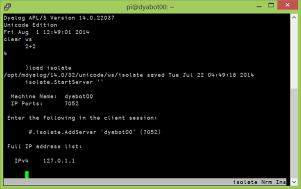
Starting an isolate server using PuTTY to run Dyalog on the robot.

Starting an isolate server on DyaBot00 using PuTTY.

Once we have an isolate server running on each robot we can take control of them from a remote session as follows:

      )load isolate
      #.isolate.AddServer 'dyabot00' (7052)      
      #.isolate.AddServer 'dyabot04' (7052)
      bots←isolate.New¨Bot Bot
      bots.Init
 dyabot00  dyabot04

Above, we create two instances of the Bot namespace. The expression Bots.Init invokes the Init function, which returns the hostname, in each isolate:

:Namespace Bot

    ∇ r←Init;pwd
      pwd←∊⎕SH'pwd' ⍝ Find out where to copy from
      #.⎕CY botws←pwd,'/DyaBot/DyaBot.dws' ⍝ copy ws
      i←⎕NEW #.DyaBot ⍬ ⍝ Make DyaBot instance    
      r←⎕SH'hostname' ⍝ Return hostname
    ∇

:EndNamespace

Next, we define a function “run” that will take a vector of dance steps as input. Each step is a character vector (because that makes editing slightly easier!) containing five numbers: The first two set the speed of one robot, the next two the speed of the other and the fifth defines the duration of the step. After each step we pause for a second, to give humans time to appreciate the spectacle:


    ∇ run cmds;data;i;cmd;z
[1]    ⎕DL 5
[2]    :For i :In ⍳≢cmds
[3]        :If ' '∨.≠cmd←i⊃cmds
[4]            data←1 0 1 0 1⊂2⊃⎕VFI cmd ⍝ Cut into 3 numeric pieces
[5]            z←bots.{i.Speed←⍵}2↑data ⋄ ⎕DL⊃¯1↑data ⋄ z←bots.(i.Speed←0)
[6]            ⎕DL 1
[7]        :EndIf
[8]    :EndFor
    ∇

Now we are ready to roll: Call the run function with a suitable array and watch the robots dance (see the video at the top)!

      ↑choreography
50  50  0   0 1.5
 0   0 50  60 1.2
50 ¯50 50 ¯50 0.3
20  80 10  70 5  
50 ¯50 50 ¯50 0.3
50  50  0   0 1.5
 0   0 50  60 1.2

      dance choreography

Join us again next week to hear what happened when Romilly came to Bramley to help wire up the accelerometer and gyro!

Aligning Diff Output

‘Bots are off limits this week so here is a story from this year’s Iverson College – a fantastic week spent in the company of a wonderful mixture of array and functional language gurus and newbies, all learning from each other. One evening, Dhru Patel presented a problem that he was working on which involved displaying the results of a “diff” side by side with the matched rows aligned. For example, the input might be:

      OLD NEW
┌────────┬────────┐
│This    │This    │
│is the  │original│
│original│is not  │
│text    │        │
└────────┴────────┘

Edited by Yoda, the text was. The selection of rows to be aligned requires finding the longest sequence of rows from the original data that matches rows in the edited data without ever skipping backwards through either sets of data. In this case, it is the original first and third row, matching the first two edited rows. We will return to how we might identify these rows in a future blog entry (meanwhile, try to grok John Scholes’ YouTube video on Depth First Searching and think about it). For now, we will provide this information as a left argument, a vector of Boolean vectors that marks the location of the matched rows:

      (1 0 1 0)(1 1 0) AlignMatched OLD NEW
┌────────┬────────┐
│This    │This    │
│is the  │        │
│original│original│
│text    │        │
│        │is not  │
└────────┴────────┘

At Iverson College there was general agreement that “there should be a non-looping solution”, and Devon McCormick immediately stated that he would bet that it involved grade (). Let us explore:

      masks←(1 0 1 0)(1 1 0)
      ⎕←matched←∊masks ⍝ The two match masks catenated together
 1 0 1 0 1 1 0 
      ⎕←origin←(≢¨OLD NEW)/0 1 ⍝ 0 for items from the old array, 1 for new
 0 0 0 0 1 1 1 
      ⎕←block←∊+\¨masks ⍝ running count of matched rows
 1 1 2 2 1 2 2   
      ⎕←data←block,(~matched),origin,OLD⍪NEW
1 0 0 This    
1 1 0 is the  
2 0 0 original
2 1 0 text    
1 0 1 This    
2 0 1 original
2 1 1 is not  

Our goal is to create an expansion mask for each argument; this is going to insert blank lines at the points where a non-matched row from the other argument is included. The next step is to reorder everything by ascending block number, and within each block move the matched rows to the front (ascending by ~matched), as follows:

      ⎕←data←data[⍋data[;1 2];]
1 0 0 This    
1 0 1 This    
1 1 0 is the  
2 0 0 original
2 0 1 original
2 1 0 text    
2 1 1 is not 

This contains all the items from both texts in the order that they would need to appear in the final results. We can extract the reordered flag vectors:

       matched←~data[;2] ⋄ origin←data[;3]

Now, (origin=0) is an expansion mask that would expand OLD to match the above, and (origin=1) would do the same for NEW:

      0 1 {(origin=⍺)⍀⍵}¨OLD NEW
┌────────┬────────┐
│This    │        │
│        │This    │
│is the  │        │
│original│        │
│        │original│
│text    │        │
│        │is not  │
└────────┴────────┘

To align the matched rows, we need to eliminate inserted blanks that correspond to matched rows from the other side:

      0 1{((~matched∧origin≠⍺)/origin=⍺)⍀⍵}¨OLD NEW
┌────────┬────────┐
│This    │This    │
│is the  │        │
│original│original│
│text    │        │
│        │is not  │
└────────┴────────┘

In the final function, which collects the relevant lines of code from our experiments, we do not create the temporary “data” matrix, but reorder the origin and matched vectors individually – and instead of doing grade up on a two-column matrix, we compute an integer vector that will sort by descending matched within ascending block (because we know that grade up on a simple small-range integer vector will run like greased lightning):

 AlignMatched←{                ⍝ align matched rows of 1⊃⍵ and 2⊃⍵
     matched←∊⍺                ⍝ matches are marked by 1⊃⍺ and 2⊃⍺
     origin←(≢¨⍵)/0 1          ⍝ identify origin of items in matched (0=old. 1=new)
     block←∊+\¨⍺               ⍝ running count of matched rows
     order←⍋(2×block)-matched  ⍝ Order so matching rows are adjacent and order of
     (origin matched)←(⊂⊂order)⌷¨origin matched ⍝ items following matched row is preserved
     0 1{((~matched∧origin≠⍺)/origin=⍺)⍀⍵}¨⍵ ⍝ Expand exluding matched from "other" list
 }


Reviving Lost Arts

The algorithm above makes use of techniques that were well-known in APL circles in the 1980s, but atrophied after nested arrays arrived on the scene and applications tended to keep parts of the data in separate leaves of an array rather than using simple data structures.

If you would like to read up on some of the old techniques, you might enjoy browsing the FinnAPL Idiom Library, and Bob Smith’s immortal Boolean Functions and Techniques. Although nested arrays might have made them a little less relevant in the 90s and 00s, the search for high-performance parallel solutions could bring them back, as explained in this session from Dyalog ’12, on Segmented Scans and Nested Data Parallelism by Andrzej Filinski.