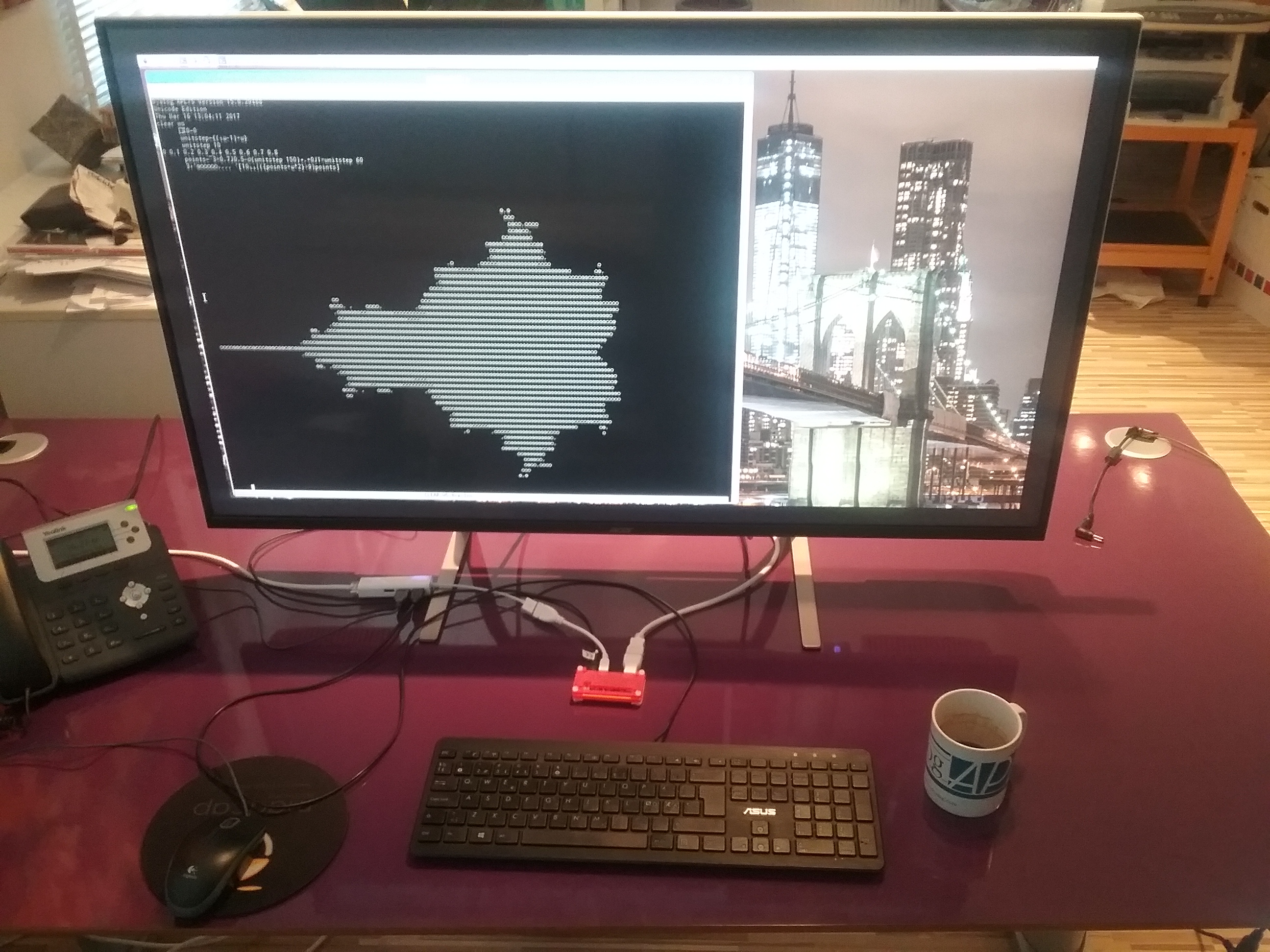
Calculation v Look-Up

(⎕io←0 and timings are done in Dyalog version 15.0.)

Table Look-Up

Some functions can be computed faster by table look-up than a more traditional and more conventional calculation. For example:

      b←?1e6⍴2

      cmpx '*b' '(*0 1)[b]'
 *b        → 1.32E¯2 |   0% ⎕⎕⎕⎕⎕⎕⎕⎕⎕⎕⎕⎕⎕⎕⎕⎕⎕⎕⎕⎕⎕⎕⎕⎕⎕⎕⎕⎕⎕⎕
 (*0 1)[b] → 1.23E¯3 | -91% ⎕⎕⎕

Some observations about this benchmark:

(a) The advantage of table look-up depends on the time to calculate the function directly, versus the time to do indexing, ⍺[⍵] or ⍵⌷⍺, plus a small amount of time to calculate the function on a (much) smaller representative set.

Indexing is particularly efficient when the indices are boolean:

      bb←b,1
      bi←b,2
      cmpx '2 3[bb]' '2 3 3[bi]'
 2 3[bb]   → 1.12E¯4 |    0% ⎕⎕⎕⎕⎕
 2 3 3[bi] → 7.39E¯4 | +558% ⎕⎕⎕⎕⎕⎕⎕⎕⎕⎕⎕⎕⎕⎕⎕⎕⎕⎕⎕⎕⎕⎕⎕⎕⎕⎕⎕⎕⎕⎕

bi is the same as bb except that the last element of 2 forces it to be 1-byte integers (for bi) instead of 1-bit booleans (for bb).

(b) Although the faster expression works best with 0-origin, the timing for 1-origin is similar.

      cmpx '*b' '{⎕io←0 ⋄ (*0 1)[⍵]}b'
 *b                   → 1.32E¯2 |   0% ⎕⎕⎕⎕⎕⎕⎕⎕⎕⎕⎕⎕⎕⎕⎕⎕⎕⎕⎕⎕⎕⎕⎕⎕⎕⎕⎕⎕⎕⎕
 {⎕io←0 ⋄ (*0 1)[⍵]}b → 1.22E¯3 | -91% ⎕⎕⎕

That is, if the current value of ⎕io is 1, the implementation can use a local ⎕io setting of 0.

(c) The fact that *b is currently slower than (*0 1)[b] represents a judgment by the implementers that *b is not a sufficiently common computation to warrant writing faster code for it. Other similar functions already embody the table look-up technique:

      cmpx '⍕b' '¯1↓,(2 2⍴''0 1 '')[b;]'
 ⍕b                   → 6.95E¯4 |  0% ⎕⎕⎕⎕⎕⎕⎕⎕⎕⎕⎕⎕⎕⎕⎕⎕⎕⎕⎕⎕⎕⎕⎕⎕⎕⎕⎕⎕⎕⎕
 ¯1↓,(2 2⍴'0 1 ')[b;] → 6.92E¯4 | -1% ⎕⎕⎕⎕⎕⎕⎕⎕⎕⎕⎕⎕⎕⎕⎕⎕⎕⎕⎕⎕⎕⎕⎕⎕⎕⎕⎕⎕⎕⎕

Small Domains

Table look-up works best for booleans, but it also works for other small domains such as 1-byte integers:

      i1←?1e6⍴128    ⍝ 1-byte integers

      cmpx '*i1' '(*⍳128)[i1]'
 *i1         → 1.48E¯2 |   0% ⎕⎕⎕⎕⎕⎕⎕⎕⎕⎕⎕⎕⎕⎕⎕⎕⎕⎕⎕⎕⎕⎕⎕⎕⎕⎕⎕⎕⎕⎕
 (*⍳128)[i1] → 9.30E¯4 | -94% ⎕⎕

      cmpx '○i1' '(○⍳128)[i1]'
 ○i1         → 2.78E¯3 |   0% ⎕⎕⎕⎕⎕⎕⎕⎕⎕⎕⎕⎕⎕⎕⎕⎕⎕⎕⎕⎕⎕⎕⎕⎕⎕⎕⎕⎕⎕⎕
 (○⍳128)[i1] → 9.25E¯4 | -67% ⎕⎕⎕⎕⎕⎕⎕⎕⎕⎕

In general, a table for 1-byte integers needs to have values for ¯128+⍳256. Here ⍳128 is used to simulate that in C indexing can be done on 1-byte indices without extra computation on the indices. In APL, general 1-byte indices are used as table[i1+128]; in C, the expression is (table+offset)[i].

Domains considered “small” get bigger all the time as machines come equipped with ever larger memories.

Larger Domains

Table look-up is applicable when the argument is not a substantial subset of a large domain and there is a fast way to detect that it is not.

      i4s←1e7+?1e6⍴1e5    ⍝ small-range 4-byte integers

      G←{(⊂u⍳⍵)⌷⍺⍺ u←∪⍵}

      cmpx '⍟i4s' '⍟G i4s'
 ⍟i4s   → 1.44E¯2 |   0% ⎕⎕⎕⎕⎕⎕⎕⎕⎕⎕⎕⎕⎕⎕⎕⎕⎕⎕⎕⎕⎕⎕⎕⎕⎕⎕⎕⎕⎕⎕
 ⍟G i4s → 9.59E¯3 | -34% ⎕⎕⎕⎕⎕⎕⎕⎕⎕⎕⎕⎕⎕⎕⎕⎕⎕⎕⎕⎕

The definition of G implements that the argument is not used directly as indices (as in (⊂⍵)⌷⍺⍺ u) but needed to be looked up, the u⍳⍵ in (⊂u⍳⍵)⌷⍺⍺ u. Thus both index-of and indexing are key enablers for making table look-up competitive.

§4.3 of Notation as a Tool of Thought presents a different way to distribute the results of a calculation on the “nub” (unique items). But it takes more time and space and is limited to numeric scalar results.

      H←{(⍺⍺ u)+.×(u←∪⍵)∘.=⍵}

      i4a←1e7+?1e4⍴1e3    ⍝ small-range 4-byte integers

      cmpx '⍟i4a' '⍟G i4a' '⍟H i4a'
 ⍟i4a   → 1.56E¯4 |       0%
 ⍟G i4a → 6.25E¯5 |     -60%
 ⍟H i4a → 1.78E¯1 | +113500% ⎕⎕⎕⎕⎕⎕⎕⎕⎕⎕⎕⎕⎕⎕⎕⎕⎕⎕⎕⎕⎕⎕⎕⎕⎕⎕⎕⎕⎕⎕

The benchmark is done on the smaller i4a as a benchmark on i4s founders on the ≢∪⍵ by ≢⍵ boolean matrix (for i4s, 12.5 GB = ×/ 0.125 1e5 1e6) created by H.

Mathematical Background

New Math” teaches that a function is a set of ordered pairs whose first items are unique:

*⍵: {(⍵,*⍵)|⍵∊C}      The set of all (⍵,*⍵) where is a complex number
⍟⍵: {(⍵,⍟⍵)|⍵∊C~{0}}  The set of all (⍵,⍟⍵) where is a non-zero complex number
○⍵: {(⍵,○⍵)|⍵∊C}      The set of all (⍵,○⍵) where is a complex number
⍕⍵: {(⍵,⍕⍵)|0=⍴⍴⍵}    The set of all (⍵,⍕⍵) where is a scalar

When is restricted (for example) to the boolean domain, the functions, the sets of ordered pairs, are more simply represented by enumerating all the possibilities:

*⍵: {(0,1), (1,2.71828)}
⍟⍵: {(0,Err), (1,0)}
○⍵: {(0,0), (1,3.14159)}
⍕⍵: {(0,'0'), (1,'1')}

Realized and Potential Performance Improvements

realized (available no later than 15.0)

boolean
1-byte integer
⍕ ∘.f
⍕     a∘⍕

potential (non-exhaustive list)

boolean
1-byte integer
2-byte integer
small-range 4-byte integer
* ⍟ | - ○   ! ⍳ a∘f f.g
* ⍟ | - ○ × ! ⍳ a∘f f.g ∘.f
* ⍟ | - ○ ×   ⍳ a∘f
* ⍟ |     ×

a is a scalar; f and g are primitive scalar dyadic functions.

Beauty and the Beast

beauty-and-the-beastFinally, the last accessory I ordered for my Raspberry Pi Zero (that’s the little red thing behind my keyboard) has arrived – an Acer 43″ ET430K monitor. The Zero won’t quite drive this monitor at its maximum resolution of 3840×2160 pixels, but as you can see, you get enough real estate to do real graphics with “ASCII Art” (well, Unicode Art, anyway)!

Some readers will recognise the image as the famous Mandelbrot Set, named after the mathematician Benoit Mandelbrot, who studied fractals. According to Wikipedia a fractal is a mathematical set that exhibits a repeating pattern displayed at every scale – they are interesting because they produce patterns that are very similar to things we can see around us – both in living organisms and landscapes – they seem to be part of the fundamental fabric of the universe.

Fractals are are also interesting because they produce images of staggering beauty, as you can see on the pages linked to above and one of our rotating banner pages, where a one-line form of the APL expression which produced the image is embedded:

Website_banner_MbrotW

The colourful images of the Mandelbrot set are produced by looking at a selection of points in the complex plane. For each point c, start with a value of 0 for z, repeat the computation z = c + z², and colour the point according to the number of iterations required before the function becomes “unbounded in value”.

In APL, the function for each iteration can be expressed as {c+⍵*2}, where c is the point and ⍵ (the right argument of the function) is z (initially 0, and subsequently the result of the previous iteration):

      f←{c+⍵*2} ⍝ define the function
      c←1J1     ⍝ c is 1+i (above and to the right of the set)
      (f 0)(f f 0)(f f f 0)(f f f f 0) (f f f f f 0)
1J1 1J3 ¯7J7 1J¯97 ¯9407J¯193

If you are not familiar with complex numbers, those results may look a bit odd. While complex addition just requires adding the real and the imaginary parts independently, the result of multiplication of two complex numbers (a + bi) and (c + di) is defined as (ac-db) + (bc+ad)i. Geometrically, complex multiplication is a combined stretching and rotation operation.

Typing all those f’s gets a bit tedious, fortunately APL has a power operator , a second-order function that can be used to repeatedly apply a function. We can also compute the magnitude of the result number using |:

      (|(f⍣6)0)(|(f⍣7)0)
8.853E7 7.837E15

Let’s take a look at what happens if we choose a point inside the Mandelbrot set:

      c←0.1J0.1
      {|(f⍣⍵)0}¨ 1 2 3 4 5 6 7 8 9 10
0.1414 0.1562 0.1566 0.1552 0.1547 0.1546 0.1546 0.1546 0.1546 0.1546

Above, I used an anonymous function so I could pass the number of iterations in as a parameter, and use the each operator ¨ to generate all the results up to ten iterations. In this case, we can see that the magnitude of the result stabilises, which is why the point 0.1 + 0.1i is considered to be inside the Mandelbrot set.

Points which are just outside the set will require varying numbers of applications of f before the magnitude “explodes”, and if you colour points according to how many iterations are needed and pick interesting areas along the edge of the set, great beauty is revealed.

1200px-GalaxyOfGalaxies

The above image is in the public domain and was created by Jonathan J. Dickau using ChaosPro 3.3 software, which was created by Martin Pfingstl.

Our next task is to create array of points in the complex plane. A helper function unitstep generates values between zero and 1 with a desired number of steps, so I can vary the resolution and size of the image. Using it, I can create two ranges, multiply one of them by i (0J1 in APL) and use an addition table (∘.+) to generate the array:

      ⎕io←0 ⍝ use index origin zero
      unitstep←{(⍳⍵+1)÷⍵}
      unitstep 6
0 0.1667 0.3333 0.5 0.6667 0.8333 1
      c←¯3 × 0.7J0.5 - (0J1×unitstep 6)∘.+unitstep 6
      c
¯2.1J¯1.5 ¯1.6J¯1.5 ¯1.1J¯1.5 ¯0.6J¯1.5 ¯0.1J¯1.5 0.4J¯1.5 0.9J¯1.5
¯2.1J¯1   ¯1.6J¯1   ¯1.1J¯1   ¯0.6J¯1   ¯0.1J¯1   0.4J¯1   0.9J¯1  
¯2.1J¯0.5 ¯1.6J¯0.5 ¯1.1J¯0.5 ¯0.6J¯0.5 ¯0.1J¯0.5 0.4J¯0.5 0.9J¯0.5
¯2.1      ¯1.6      ¯1.1      ¯0.6      ¯0.1      0.4      0.9     
¯2.1J00.5 ¯1.6J00.5 ¯1.1J00.5 ¯0.6J00.5 ¯0.1J00.5 0.4J00.5 0.9J00.5
¯2.1J01   ¯1.6J01   ¯1.1J01   ¯0.6J01   ¯0.1J01   0.4J01   0.9J01  
¯2.1J01.5 ¯1.6J01.5 ¯1.1J01.5 ¯0.6J01.5 ¯0.1J01.5 0.4J01.5 0.9J01.5

The result is subtracted from 0.7J0.5 (0.7 + 0.5i) to get the origin of the complex plane slightly off centre in the middle, and multiplied the whole thing by 3 to get a set of values that brackets the Mandelbrot set.

Note that APL expressions are typically rank and shape invariant, so our function f can be applied to the entire array without changes. Since our goal is only to produce ASCII art, we don’t need to count iterations, we can just compare the magnitude of the result with 9 to decide whether the point has escaped:

      9<|f 0
0 0 0 0 0 0 0
0 0 0 0 0 0 0
0 0 0 0 0 0 0
0 0 0 0 0 0 0
0 0 0 0 0 0 0
0 0 0 0 0 0 0
0 0 0 0 0 0 0
      9<|(f⍣3) 0 ⍝ Apply f 3 times
1 1 1 0 0 0 1
1 0 0 0 0 0 0
0 0 0 0 0 0 0
0 0 0 0 0 0 0
0 0 0 0 0 0 0
1 0 0 0 0 0 0
1 1 1 0 0 0 1

We can see that points around the edge start escaping after 3 iterations. Using an anonymous function again, we can observe more and more points escape, until we recognise the (very low resolution) outline of the Mandelbrot set:


      ]box on
      {((⍕⍵)@(⊂0 0))' #'[9>|(f⍣⍵)0]}¨2↓⍳9
┌───────┬───────┬───────┬───────┬───────┬───────┬───────┐
│2######│3  ### │4      │5      │6      │7      │8      │
│#######│ ######│   ### │    #  │    #  │    #  │    #  │
│#######│#######│ ##### │  #### │  #### │   ### │   ### │
│#######│#######│###### │ ##### │ ##### │ ##### │ ####  │
│#######│#######│ ##### │  #### │  #### │   ### │   ### │
│#######│ ######│   ### │    #  │    #  │    #  │    #  │
│#######│   ### │       │       │       │       │       │
└───────┴───────┴───────┴───────┴───────┴───────┴───────┘

The last example allowed me to sneak in a preview of the new “at” operator coming in Dyalog v16.0. It is a functional merge operator that I am using to insert the formatted right argument (the number of iterations) into position (0 0) of each matrix.

If I use our remote IDE (RIDE) on my Windows machine and connect to the Pi, I can have an APL session on the Pi with 3840×2160 resolution. In this example, I experimented with grey scale “colouring” the result by rounding down and capping the result at 10, and using the character ⍟ (darkest) for 0, ○ for 1-5, × for 6-9, and blank for points that “escaped”, by indexing into an array of ten characters:

      '⍟○○○○○×××× '[10⌊⌊|(f⍣9)c]

Who needs OpenGL?! (click on the image to enlarge)

mandelbrot-ride4

Charting Reaction Times on the Raspberry Pi

Earlier this week I collected some reaction timer data on my Pi using the BBC micro:bit as an input device. I only produced an “ASCII art” chart at the time:

      times←ReactionTimer.Play
      times
251 305 294 415 338 298 294 251 378
      ReactionTimer.AsciiChart times
425| 
400|    * 
375|         *
350+ 
325|     * 
300|  * 
275|   *  ** 
250+ *      * 

Retro is back in style – but of course I should point out that we can produce “proper” graphics using SharpPlot, a cross-platform graphics package that is included with Dyalog APL on all platforms. I’ve enhanced the ReactionTimer namespace with a function called SPHistogram. If you are using RIDE as the front end to APL on the Pi, this will render output from SharpPlot in a window:

    ReactionTimer.SPHistogram times

Reaction Time Histogram

The original ASCII chart simply plotted the observations in the order that they occurred. Above, the shaded areas show how many observations there were in each bucket (2 between 250ms and 275ms, 3 between 275ms and 300ms, and so on). At the same time, the individual observations can be seen along the X axis as vertical red lines. It is a little unfortunate that, presumably due to some artifact of the timing process, the values 251 and 294 occur twice – and these lines are drawn on top of each other.

The example highlights one of the things that makes SharpPlot a bit special: We have overlaid a histogram showing the frequency of reactions in each bucket, and used a “scatterplot” to where the Y value is always 0, to mark the individual observations along the X axis.

     ∇ SPHistogram times;heading;renderHtml;sp;svg;z 
[1]   heading←'Reaction Times' 
[2]   renderHtml←3500⌶ ⍝ Render HTML in Window 
[3] 
[4]   :If 0=⎕NC'#.SharpPlot' ⋄ #.⎕CY'sharpplot.dws' ⋄ :EndIf
[5] 
[6]   sp←⎕NEW #.SharpPlot(432 250) 
[7]   sp.Heading←heading 
[8] 
[9]   ⍝ Draw histogram 
[10]  sp.ClassInterval←25 
[11]  sp.SetXTickMarks 25 
[12]  sp.HistogramStyle←#.HistogramStyles.SurfaceShading 
[13]  sp.SetFillStyles #.FillStyle.Opacity30 
[14]  sp.DrawHistogram⊂times 
[15] 
[16]  ⍝ Add observations using ScatterPlot 
[17]  sp.SetMarkers #.Marker.UpTick 
[18]  sp.SetPenWidths 1 
[19]  sp.SetMarkerScales 3 
[20]  sp.DrawScatterPlot(times×0)(times) 
[21] 
[22]  ⍝ Render SVG and display in window 
[23]  svg←sp.RenderSvg #.SvgMode.FixedAspect 
[24]  z←heading renderHtml svg 
     ∇ 

Hopefully the code is more or less self-explanatory, but if you’d like to learn more about SharpPlot there is excellent documentation at http://sharpplot.com. The documentation is actually written for C# users, but there is an illustration of how to translate the documentation to APL (and VB) at http://www.sharpplot.com/Languages.htm.

micro:bit Reaction Timer in APL on the Pi and BBC micro:bit

BBC micro:bit displaying a happy face

BBC micro:bit displaying a happy face

I have a bit of a cold today, so I decided that instead of hopping in an icy car and driving to the office in order to spend the day drinking coffee and answering e-mail, I should stay at home, turn up the radiators, make lots of tea (with honey!) and have some fun writing code on my Raspberry Pi! Can there be a better way to ensure a speedy recovery?

By the way, if you are already a user of Dyalog APL but you haven’t got a Pi yet, you should read The APLer’s Quick-start Guide to the Raspberry Pi, which Romilly Cocking completed a few days ago. This explains what your options are for buying hardware, and how to get going with a free copy of Dyalog APL. If you don’t read it now, your cold may be over before all the bits are delivered, so hurry up!

I wasn’t feeling THAT energetic this morning, so I decided to ease back into things by trying to replicate Romilly’s reaction timer, which is written in MicroPython. To begin with, I extended the microbit class that I developed for the Morse code display function with a few new methods to cover the API calls that allow me to check the state of the two buttons on each side of the micro:bit display (see the image above).

First, I added a method called is_true, which takes a MicroPython expression as an argument, evaluates it using the PyREPL function, and returns 0 or 1 depending on whether the expression returns False or True (and fails if it returns something else):

 ∇ r←is_true expr;t;z
 :Access Public
 r←1⊃t←'True' 'False'∊⊂z←PyREPL expr
 :If ~∨/t ⋄ ⎕←'True/False expected, got: ',z ⋄ ∘∘∘ ⋄ :EndIf
 ∇

This is a useful building block, which allows the simple construction of functions like was_pressed, which takes ‘a’ or ‘b’ as an argument and tells you whether the button in question has been pressed since you last asked:

∇ r←was_pressed button
 :Access Public
 r←is_true 'button_',button,'.was_pressed()' 
∇

Once this is done, writing the Play function in the ReactionTimer namespace is easy, you can find the rest of the code on GitHub. The APL version is different from the MicroPython version in that – once the user presses button B and stops the game – the reaction times (in milliseconds) are returned as an integer vector. So now we can have some fun with data!

In the spirit of the micro:bit, I thought I’d produce a low tech character based chart, trying to remember the skills that were start-of-the-art when I started using APL. The AsciiChart function in the ReactionTimer namespace takes a vector of timings as the right argument, and produces a chart:

      times←ReactionTimer.Play
      times
251 305 294 415 338 298 294 251 378
      ReactionTimer.AsciiChart times
425| 
400|    * 
375|         *
350+ 
325|     * 
300|  * 
275|   *  ** 
250+ *      * 

The code (which is also on GitHub) is listed below. Because this is a pure function, I used the modern dfns style of function definition rather than the old style procedural form that I’ve used for the object oriented code. The function works by allocating each value to a bucket of the size defined by the variable scale. The fun part is the use of the outer product with equals (∘.=) between the list of buckets on the left (rb) and the scaled values on the right (⌊⍵÷scale) – and then using this Boolean array to index into a two-element character vector to produce the chart. The rest is scaling calculations and finally decorating with “tik marks”:

 AsciiChart←{
     scale←25 ⍝ size of each row
     tiks←4 ⍝ tik spacing
     (max min)←(⌈/ , ⌊/) ⍵ ⍝ maximum and minimum
     base←⌊min÷scale ⍝ round down to nearest scale unit
     rb←base+0,⍳⌈(max-min)÷scale ⍝ row base values
     r←' *'[1+rb∘.=⌊⍵÷scale] ⍝ our chart
     r←((≢rb)⍴'+',(tiks-1)⍴'|'),' ',r ⍝ add tiks
     r←(⍕⍪rb×scale),r ⍝ add base values
     ⊖r ⍝ low values last (humans!)
 }

Although I might be feeling better tomorrow, I expect to be back soon. I have a couple of plastic bags full of resistors, LEDs, potentiometers and cameras (yes, plural) that I have not opened yet!

50847534

⎕io←0 throughout.

I was re-reading A Mathematician’s Apology before recommending it to Suki Tekverk, our summer intern, and came across a statement that the number of primes less than 1e9 is 50847478 (§14, page 23). The function pco from the dfns workspace does computations on primes; ¯1 pco n is the number of primes less than n:

      )copy dfns pco

      ¯1 pco 1e9
50847534

The two numbers 50847478 and 50847534 cannot both be correct. A search of 50847478 on the internet reveals that it is incorrect and that 50847534 is correct. 50847478 is erroneously cited in various textbooks and even has a name, Bertelsen’s number, memorably described by MathWorld as “an erroneous name erroneously given the erroneous value of π(1e9) = 50847478.”

Although several internet sources give 50847534 as the number of primes less than 1e9, they don’t provide a proof. Relying on them would be doing the same thing — arguing from authority — that led other authors astray, even if it is the authority of the mighty internet. Besides, I’d already given Suki, an aspiring mathematician, the standard spiel about the importance of proof.

How do you prove the 50847534 number? One way is to prove correct a program that produces it. Proving pco correct seems daunting — it has 103 lines and two large tables. Therefore, I wrote a function from scratch to compute the number of primes less than , a function written in a way that facilitates proof.

sieve←{
  b←⍵⍴{∧⌿↑(×/⍵)⍴¨~⍵↑¨1}2 3 5
  b[⍳6⌊⍵]←(6⌊⍵)⍴0 0 1 1 0 1
  49≥⍵:b
  p←3↓{⍵/⍳⍴⍵}∇⌈⍵*0.5
  m←1+⌊(⍵-1+p×p)÷2×p
  b ⊣ p {b[⍺×⍺+2×⍳⍵]←0}¨ m
}

      +/ sieve 1e9
50847534

sieve ⍵ produces a boolean vector b with length such that b/⍳⍴b are all the primes less than . It implements the sieve of Eratosthenes: mark as not-prime multiples of each prime less than ⍵*0.5; this latter list of primes obtains by applying the function recursively to ⌈⍵*0.5. Some obvious optimizations are implemented:

  • Multiples of 2 3 5 are marked by initializing b with ⍵⍴{∧⌿↑(×/⍵)⍴¨~⍵↑¨1}2 3 5 rather than with ⍵⍴1.
  • Subsequently, only odd multiples of primes > 5 are marked.
  • Multiples of a prime to be marked start at its square.

Further examples:

      +/∘sieve¨ ⍳10
0 0 0 1 2 2 3 3 4 4

      +/∘sieve¨ 10*⍳10
0 4 25 168 1229 9592 78498 664579 5761455 50847534

There are other functions which are much easier to prove correct, for example, sieve1←{2=+⌿0=(⍳3⌈⍵)∘.|⍳⍵}. However, sieve1 requires O(⍵*2) space and sieve1 1e9 cannot produce a result with current technology. (Hmm, a provably correct program that cannot produce the desired result …)

We can test that sieve is consistent with pco and that pco is self-consistent. pco is a model of the p: primitive function in J. Its cases are:
   pco n   the n-th prime
¯1 pco n   the number of primes less than n
 1 pco n   1 iff n is prime
 2 pco n   the prime factors and exponents of n
 3 pco n   the prime factorization of n
¯4 pco n   the next prime < n
 4 pco n   the next prime > n
10 pco r,s a boolean vector b such that r+b/⍳⍴b are the primes in the half-open interval [r,s).

      ¯1 pco 10*⍳10      ⍝ the number of primes < 1e0 1e1 ... 1e9
0 4 25 168 1229 9592 78498 664579 5761455 50847534

      +/ 10 pco 0 1e9    ⍝ sum of the sieve between 0 and 1e9
50847534
                         ⍝ sum of sums of 10 sieves
                         ⍝ each of size 1e8 from 0 to 1e9
      +/ t← {+/10 pco ⍵+0 1e8}¨ 1e8×⍳10
50847534
                         ⍝ sum of sums of 1000 sieves
                         ⍝ each of size 1e6 from 0 to 1e9
      +/ s← {+/10 pco ⍵+0 1e6}¨ 1e6×⍳1000
50847534

      t ≡ +/ 10 100 ⍴ s
1
                         ⍝ sum of sums of sieves with 1000 randomly
                         ⍝ chosen end-points, from 0 to 1e9
      +/ 2 {+/10 pco ⍺,⍵}/ 0,({⍵[⍋⍵]}1000?1e9),1e9
50847534

      ¯1 pco 1e9         ⍝ the number of primes < 1e9
50847534
      pco 50847534       ⍝ the 50847534-th prime
1000000007
      ¯4 pco 1000000007  ⍝ the next prime < 1000000007
999999937
      4 pco 999999937    ⍝ the next prime > 999999937
1000000007     
      4 pco 1e9          ⍝ the next prime > 1e9
1000000007

                         ⍝ are 999999937 1000000007 primes?
      1 pco 999999937 1000000007
1 1
                         ⍝ which of 999999930 ... 1000000009
                         ⍝ are prime?
      1 pco 999999930+4 20⍴⍳80
0 0 0 0 0 0 0 1 0 0 0 0 0 0 0 0 0 0 0 0
0 0 0 0 0 0 0 0 0 0 0 0 0 0 0 0 0 0 0 0
0 0 0 0 0 0 0 0 0 0 0 0 0 0 0 0 0 0 0 0
0 0 0 0 0 0 0 0 0 0 0 0 0 0 0 0 0 1 0 1

      +/∘sieve¨ 999999937 1000000007 ∘.+ ¯1 0 1
50847533 50847533 50847534
50847534 50847534 50847535

A Memo Operator

Abstract

Some functions are simply stated and easily understood as multiply-recursive functions. For example, the Fibonacci numbers are {1≥⍵:⍵ ⋄ (∇ ⍵-2)+∇ ⍵-1}. A drawback of multiple recursion is abysmal performance even for moderate-sized arguments, consequently motivating resorts to circumlocutions. The memo operator addresses the performance problem and restores multiple recursion to the toolkit of thought. We present a memo operator modelled as a 6-line d-operator.

⎕io←0 throughout.

The Man Who Knew Infinity

Jay sent out an e-mail asking who would be interested to go see the film The Man Who Knew Infinity. Fiona’s response: “Ah, Mr. 1729; I’m in.” John was game, and so was I.

The Number of Partitions
Nick found an essay by Stephen Wolfram on Ramanujan written on occasion of the film, wherein Wolfram said:

A notable paper [Ramanujan] wrote with Hardy concerns the partition function (PartitionsP in the Wolfram Language) that counts the number of ways an integer can be written as a sum of positive integers. …

In Ramanujan’s day, computing the exact value of PartitionsP[200] was a big deal — and the climax of his paper. But now, thanks to Ramanujan’s method, it’s instantaneous:

In[1]:= PartitionsP[200]
Out[1]= 3 972 999 029 388

A partition of a non-negative integer n is a vector v of positive integers such that n = +/v, where the order in v is not significant. For example, the partitions of the first seven non-negative integers are:

┌┐
││
└┘
┌─┐
│1│
└─┘
┌─┬───┐
│2│1 1│
└─┴───┘
┌─┬───┬─────┐
│3│2 1│1 1 1│
└─┴───┴─────┘
┌─┬───┬───┬─────┬───────┐
│4│3 1│2 2│2 1 1│1 1 1 1│
└─┴───┴───┴─────┴───────┘
┌─┬───┬───┬─────┬─────┬───────┬─────────┐
│5│4 1│3 2│3 1 1│2 2 1│2 1 1 1│1 1 1 1 1│
└─┴───┴───┴─────┴─────┴───────┴─────────┘
┌─┬───┬───┬─────┬───┬─────┬───────┬─────┬───────┬─────────┬───────────┐
│6│5 1│4 2│4 1 1│3 3│3 2 1│3 1 1 1│2 2 2│2 2 1 1│2 1 1 1 1│1 1 1 1 1 1│
└─┴───┴───┴─────┴───┴─────┴───────┴─────┴───────┴─────────┴───────────┘

Can we compute the partition counting function “instantaneously” in APL?

We will use a recurrence relation derived from the pentagonal number theorem, proved by Euler more than 160 years before Hardy and Ramanujan:

equation (11) in http://mathworld.wolfram.com/PartitionFunctionP.html. In APL:

      pn  ← {0≥⍵:0=⍵ ⋄ -/+⌿∇¨rec ⍵}
      rec ← {⍵ - (÷∘2 (×⍤1) ¯1 1 ∘.+ 3∘×) 1+⍳⌈0.5*⍨⍵×2÷3}

      pn¨0 1 2 3 4 5 6
1 1 2 3 5 7 11

      pn 30
5604

Warning: don’t try pn 200 because that would take a while! Why? pn 200 would engender pn being applied to each element of rec 200 and:

   rec 200
199 195 188 178 165 149 130 108 83 55 24 ¯10
198 193 185 174 160 143 123 100 74 45 13 ¯22

Each of the non-negative values would itself engender further recursive applications.

A Memo Operator

I recalled from J the memo adverb (monadic operator) M. Paraphrasing the J dictionary: f M is the same as f but may keep a record of the arguments and results for reuse. It is commonly used for multiply-recursive functions. Sounds like just the ticket!

The functionistas had previously implemented a (dyadic) memo operator. The version here is more restrictive but simpler. The restrictions are as follows:

  • The cache is constructed “on the fly” and is discarded once the operand finishes execution.
  • The operand is a dfn {condition:basis ⋄ expression} where none of condition, base and expression contain a and recursion is denoted by in expression
  • The arguments are scalar integers.
  • The operand function does not have ¯1 as a result.
  • A recursive call is on a smaller integer.

With these restrictions, our memo operator can be defined as follows:

M←{
 f←⍺⍺
 i←2+'⋄'⍳⍨t←3↓,⎕CR'f'
 0=⎕NC'⍺':⍎' {T←(1+  ⍵)⍴¯1 ⋄  {',(i↑t),'¯1≢T[⍵]  :⊃T[⍵]   ⋄ ⊃T[⍵]  ←⊂',(i↓t),'⍵}⍵'
          ⍎'⍺{T←(1+⍺,⍵)⍴¯1 ⋄ ⍺{',(i↑t),'¯1≢T[⍺;⍵]:⊃T[⍺;⍵] ⋄ ⊃T[⍺;⍵]←⊂',(i↓t),'⍵}⍵'
}

      pn M 10
42

      pn 10
42

Obviously, the lines in M are crucial. When the operand is pn, the expression which is executed is as follows; the characters inserted by M are shown in red.

{T←(1+⍵)⍴¯1 ⋄ {0≥⍵:0=⍵ ⋄ ¯1≢T[⍵]:⊃T[⍵] ⋄ ⊃T[⍵]←⊂-/+⌿∇¨rec ⍵}⍵}

The machinations produce a worthwhile performance improvement:

      pn M 30
5604
      cmpx 'pn M 30'
3.94E¯4
      cmpx 'pn 30'
4.49E1 
      4.49e1 ÷ 3.94e¯4
113959

That is, pn M 30 is faster than pn 30 by a factor of 114 thousand.

Can APL compute pn M 200 “instantaneously”? Yes it can, for a suitable definition of “instantaneous”.

      cmpx 'm←pn M 200'
4.47E¯3
      m
3.973E12
      0⍕m
 3972999029388

M also works on operands which are anonymous, dyadic, or have non-scalar results.

Fibonacci Numbers

   fib←{1≥⍵:⍵ ⋄ (∇ ⍵-2)+∇ ⍵-1}

   fib¨ ⍳15
0 1 1 2 3 5 8 13 21 34 55 89 144 233 377
   fib M¨ ⍳15
0 1 1 2 3 5 8 13 21 34 55 89 144 233 377

   cmpx 'fib 30'
1.45E0 
   cmpx 'fib M 30'
1.08E¯4

Anonymous function:

      {1≥⍵:⍵ ⋄ (∇ ⍵-2)+∇ ⍵-1}M¨ ⍳15
0 1 1 2 3 5 8 13 21 34 55 89 144 233 377

Combinations
⍺ comb ⍵ produces a matrix of all the size- combinations of ⍳⍵. The algorithm is from the venerable APL: An Interactive Approach by Gilman and Rose.

      comb←{(⍺≥⍵)∨0=⍺:((⍺≤⍵),⍺)⍴⍳⍺ ⋄ (0,1+(⍺-1)∇ ⍵-1)⍪1+⍺ ∇ ⍵-1}

      3 comb 5
0 1 2
0 1 3
0 1 4
0 2 3
0 2 4
0 3 4
1 2 3
1 2 4
1 3 4
2 3 4

      3 (comb ≡ comb M) 5
1

      cmpx '8 comb M 16' '8 comb 16'
  8 comb M 16 → 1.00E¯3 |     0% ⎕                             
  8 comb 16   → 3.63E¯2 | +3526% ⎕⎕⎕⎕⎕⎕⎕⎕⎕⎕⎕⎕⎕⎕⎕⎕⎕⎕⎕⎕⎕⎕⎕⎕⎕⎕⎕⎕⎕⎕

A faster comb is possible without a memo operator, but it’s not easy. (See for example section 4.1 of my APL87 paper.) A memo operator addresses the performance problem with multiple recursion and restores it to the toolkit of thought.

Presented at the BAA seminar at the Royal Society of Arts on 2016-05-20