Dyalog ’18 Videos, Week 6

Happy New Year – and Welcome to the 6th week of Dyalog ’18 video releases!

If you enjoy geometry, 2019 starts with a couple of real treats; one which builds up to the use of complex numbers just before the end, and another which starts with them and moves on to Quaternions. Alternatively, if you think vectors and matrices containing imaginary numbers are a bit esoteric, what could be more “down to earth” than taking a look at various ways to efficiently extract data from Excel spreadsheets? Finally, we have a talk on a Theory of Everything, which will obviously interest everyone!

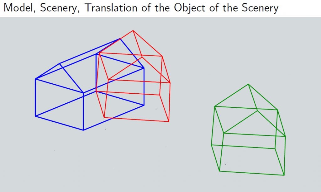
Returning to the maths: Nic Delcros asks a seemingly trivial question about the number of dimensions of a vector. As any APLer knows, a vector is a list of numbers and, therefore, has 1 dimension, but of course the numbers in a vector nearly always represent a structure of higher dimensionality. Nic takes us on an entertaining exploration of the case where the numbers represent a dynamic event, where one of the dimensions is time – punctuated with beautiful images.

Dieter Kilsch from the University of Applied Sciences (Technische Hochschule) in Bingen obviously enjoys teaching mathematics! In this talk, he actually managed to make me think that I had some insight into why the Irish mathematician William Hamilton invented the Hamiltonian number system (which is populated by Quaternions), and how it allows us to do algebra on points in a 3-dimensional space, similar to the way complex numbers work for 2 dimensions. For example, Quaternions can be used as a tool of thought and computation for image recognition!

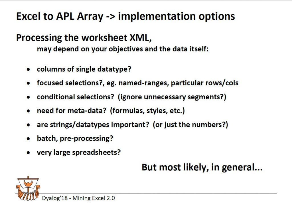
Returning to the very real world, Richard Procter is back with an updated talk on “Excel Mining”, following on from his talk at Dyalog ’15 in Sicily. Like many of us, he frequently needs to load data which originates in Microsoft Excel into APL for processing – and sometimes write back to Excel. Richard has tried a variety of different techniques and provides a list of questions that might decide which technique to use in a given scenario (and performance measurements as well).

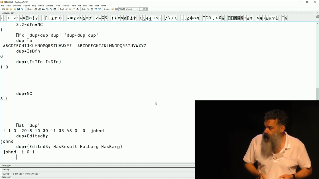
It should be no big surprise that John Daintree’s big TOE is not something he needs to take a shoe off to demonstrate. Rather, the Theory Of Everything is a unifying idea that might one day replace a large number of system functions, “root methods” and I-Beams which currently allow programmers to ask questions about the Universe that they are running in. The result will hopefully be a system that is more powerful, but simpler and much more self-documenting than the collection of tools that it would replace.

Summary of this week’s videos:


Progressive Index-Of

⎕io=0 is assumed throughout.

A recent Forum post motivated investigations into the progressive index-of functions in the FinnAPL Idiom Library:

pix  ← {((⍴⍺)⍴⍋⍋⍺⍳⍺,⍵) ⍳ ((⍴⍵)⍴⍋⍋⍺⍳⍵,⍺)}   ⍝ FinnAPL Idiom 1
pixa ← {((⍋⍺⍳⍺,⍵)⍳⍳⍴⍺) ⍳ ((⍋⍺⍳⍵,⍺)⍳⍳⍴⍵)}   ⍝ FinnAPL Idiom 5

In this note, we:

  • explain what is progressive index-of
  • explain why the two functions work
  • investigate the performance of the two functions
  • provide a more general solution

Progressive Index-Of

Progressive index-of is like index-of () except that each find “uses up” the target of that find. There are no duplicates in the result with the possible exception of ≢⍺ (for “not found”). Thus:

      x←'mississippi'
      y←'dismiss'

      x pix y
11 1 2 0 4 3 5

The following chart illustrates a step-by-step derivation of each progressive index:

0 1 2 3 4 5 6 7 8 9 10

m i s s i s s i p p  i      d i s m i s s
                           11
m i s s i s s i p p  i      d i s m i s s
                           11 1
m i s s i s s i p p  i      d i s m i s s
                           11 1 2
m i s s i s s i p p  i      d i s m i s s
                           11 1 2 0
m i s s i s s i p p  i      d i s m i s s
                           11 1 2 0 4
m i s s i s s i p p  i      d i s m i s s
                           11 1 2 0 4 3
m i s s i s s i p p  i      d i s m i s s
                           11 1 2 0 4 3 5

It is possible to compute the progressive index without looping or recursion, as the two FinnAPL functions demonstrate.

Why It Works

The basic idea of ⍺ pix ⍵ is to substitute for each item of and an equivalent representative, collectively c and d, whence the result obtains as c⍳d. The equivalent representative used here is ranking, specifically the ranking of the indices in .

The ranking of an array is a permutation of order ≢⍵. The smallest major cell is assigned 0; the next smallest is assigned 1; and so on. Ties are resolved by favoring the earlier-occurring cell. The ranking can be computed by ⍋⍋⍵. For example:

      x ⍪ ⍉⍪ ⍋⍋x
m i s s i s  s i p p i
4 0 7 8 1 9 10 2 5 6 3

      y ⍪ ⍉⍪ ⍋⍋y
d i s m i s s
0 1 4 3 2 5 6

⍺ pix ⍵ works on two different rankings of indices in :

⍋⍋⍺⍳⍺,⍵    rankings of indices in of and , favoring
⍋⍋⍺⍳⍵,⍺    rankings of indices in of and , favoring

The first ⍴⍺ items of the former are those for and the first ⍴⍵ of the latter are those for , and we get

pix ← {((⍴⍺)⍴⍋⍋⍺⍳⍺,⍵) ⍳ ((⍴⍵)⍴⍋⍋⍺⍳⍵,⍺)}

The second version depends on the following properties of permutations. Let p be a permutation. Then p[⍋p] ←→ ⍳≢p, the identity permutation, and therefore ⍋p is the inverse of p. Furthermore, p[p⍳⍳≢p] ←→ ⍳≢p and so p⍳⍳≢p is also the inverse of p. The inverse is unique (that’s why it’s called the inverse), therefore ⍋p ←→ p⍳⍳≢p.

      p←97?97         ⍝ a random permutation

      p[⍋p]    ≡ ⍳≢p
1
      p[p⍳⍳≢p] ≡ ⍳≢p
1
      (⍋p)     ≡ p⍳⍳≢p
1

The two rankings are permutations (because the leftmost functions are ) and we just need the first ⍴⍺ items of the former and the first ⍴⍵ items of the latter. Thus:

pixa ← {((⍋⍺⍳⍺,⍵)⍳⍳⍴⍺) ⍳ ((⍋⍺⍳⍵,⍺)⍳⍳⍴⍵)}

Performance

We note that both versions of pix contain the expressions ⍺⍳⍺,⍵ and ⍺⍳⍵,⍺, but the latter is just a rotation of the former. Thus:

pixb ← {i←⍺⍳⍺,⍵ ⋄ ((⍴⍺)⍴⍋⍋i) ⍳ ((⍴⍵)⍴⍋⍋(⍴⍺)⌽i)}
pixc ← {i←⍺⍳⍺,⍵ ⋄ ((⍋i)⍳⍳⍴⍺) ⍳ ((⍋(⍴⍺)⌽i)⍳⍳⍴⍵)}

Which is faster? The answer may surprise.

      x←?1e6⍴3e5
      y←?2e5⍴3e5

      cmpx 'x pixb y' 'x pixc y'
  x pixb y → 9.15E¯2 |  0% ⎕⎕⎕⎕⎕⎕⎕⎕⎕⎕⎕⎕⎕⎕⎕⎕⎕⎕⎕⎕⎕⎕⎕⎕⎕⎕⎕⎕⎕⎕
  x pixc y → 9.21E¯2 |  0% ⎕⎕⎕⎕⎕⎕⎕⎕⎕⎕⎕⎕⎕⎕⎕⎕⎕⎕⎕⎕⎕⎕⎕⎕⎕⎕⎕⎕⎕⎕

A few factors about the Dyalog APL interpreter are relevant to this performance:

  • Computing ⍺⍳⍵,⍺ as a rotation of an already computed i←⍺⍳⍺,⍵ produces a worthwhile speed-up, although only on a relatively small part of the overall computation.
          i←x⍳x,y
          cmpx '(⍴x)⌽i' 'x⍳y,x'
      (⍴x)⌽i → 5.00E¯4 |     0% ⎕⎕                            
      x⍳y,x  → 7.19E¯3 | +1337% ⎕⎕⎕⎕⎕⎕⎕⎕⎕⎕⎕⎕⎕⎕⎕⎕⎕⎕⎕⎕⎕⎕⎕⎕⎕⎕⎕⎕⎕⎕
    
  • Both and have special code for small range data.
          s←?1e6⍴5e5           ⍝ small range
          t←s ⋄ t[t⍳⌈/t]←2e9   ⍝ large range
    
          cmpx 's⍳s' 't⍳t'
      s⍳s → 5.87E¯3 |    0% ⎕⎕⎕⎕⎕⎕⎕⎕⎕                     
      t⍳t → 2.00E¯2 | +240% ⎕⎕⎕⎕⎕⎕⎕⎕⎕⎕⎕⎕⎕⎕⎕⎕⎕⎕⎕⎕⎕⎕⎕⎕⎕⎕⎕⎕⎕⎕
    
          cmpx '⍋s' '⍋t'
      ⍋s → 3.25E¯2 |   0% ⎕⎕⎕⎕⎕⎕⎕⎕⎕⎕⎕⎕⎕⎕⎕⎕⎕⎕⎕⎕⎕⎕⎕⎕⎕     
      ⍋t → 3.84E¯2 | +18% ⎕⎕⎕⎕⎕⎕⎕⎕⎕⎕⎕⎕⎕⎕⎕⎕⎕⎕⎕⎕⎕⎕⎕⎕⎕⎕⎕⎕⎕⎕
    
  • ⍋⍵ has special code when is a permutation.
          p←1e6?1e6           ⍝ p is a permutation
          q←p ⋄ q[999999]←⊃q  ⍝ q is not; both are small-range
    
          cmpx '⍋p' '⍋q'
      ⍋p → 5.81E¯3 |    0% ⎕⎕⎕                           
    * ⍋q → 5.71E¯2 | +882% ⎕⎕⎕⎕⎕⎕⎕⎕⎕⎕⎕⎕⎕⎕⎕⎕⎕⎕⎕⎕⎕⎕⎕⎕⎕⎕⎕⎕⎕⎕
    
  • We saw previously that if p is a permutation then ⍋p ←→ p⍳⍳⍴p. The special code for ⍋p makes the two expressions run at roughly the same speed. The slight advantage for ⍋⍋x versus (⍋x)⍳⍳⍴x would increase if and when ⍋⍋ is recognized as an idiom.
          cmpx '⍋p' 'p⍳⍳⍴p'
      ⍋p    → 6.02E¯3 |  0% ⎕⎕⎕⎕⎕⎕⎕⎕⎕⎕⎕⎕⎕⎕⎕⎕⎕⎕⎕⎕⎕⎕⎕⎕⎕⎕⎕   
      p⍳⍳⍴p → 6.57E¯3 | +9% ⎕⎕⎕⎕⎕⎕⎕⎕⎕⎕⎕⎕⎕⎕⎕⎕⎕⎕⎕⎕⎕⎕⎕⎕⎕⎕⎕⎕⎕⎕
    
          cmpx '⍋⍋x' '(⍋x)⍳⍳⍴x'
      ⍋⍋x      → 3.16E¯2 |  0% ⎕⎕⎕⎕⎕⎕⎕⎕⎕⎕⎕⎕⎕⎕⎕⎕⎕⎕⎕⎕⎕⎕⎕⎕⎕⎕⎕⎕⎕ 
      (⍋x)⍳⍳⍴x → 3.25E¯2 | +2% ⎕⎕⎕⎕⎕⎕⎕⎕⎕⎕⎕⎕⎕⎕⎕⎕⎕⎕⎕⎕⎕⎕⎕⎕⎕⎕⎕⎕⎕⎕


A General Solution

Index-of works on cells rather than just scalars. Likewise, progressive index-of can also be extended to work on cells. The core algorithm remains the same. The generalization obtains by first reshaping to have the same rank as (having major cells with the same shape), applying the core algorithm, and then reshaping its result to have the same leading shape as the original . Thus:

pixd←{
  m←≢⍺
  r←0⌊1-⍴⍴⍺
  n←×/r↓⍴⍵
  i←⍺⍳⍺⍪(n,1↓⍴⍺)⍴⍵
  (r↓⍴⍵) ⍴ ((⍋i)⍳⍳m) ⍳ ((⍋m⌽i)⍳⍳n)
}

   xx              yy
mmmm            dddd
iiii            iiii
ssss            ssss
ssss            mmmm
iiii            iiii
ssss            ssss
iiii     
pppp     
pppp                                  x
iiii                               mississippi

   ⍴xx             ⍴yy                y
11 4            7 4                dismiss

   xx pixd yy                         x pixd y
11 1 2 0 4 3 5                     11 1 2 0 4 3 5

   xx pixd 3 5 4⍴yy                   x pixd 3 5⍴y
11  1  2  0  4                     11  1  2  0  4
 3  5 11  7  6                      3  5 11  7  6
11 10 11 11 11                     11 10 11 11 11

Postscript
After having written the above, I discovered an alternative exposition on progressive index-of by Bob Smith entitled Anatomy of an Idiom. Adám Brudzewsky has produced a Stack Exchange lesson and a Jupyter Notebook based on Smith’s text.

There is also an exposition in J on the same topic, with a more verbose but easier-to-understand derivation.

Is it Sorted?

Motivation

I have been working on the Dyalog APL quicksort implementation. The following programming puzzle arose in the process of doing the QA for this work.

is a simple array. Write a function sorted, without using or , such that sorted ⍵ is 1 if is sorted in ascending order and 0 otherwise.

The point about not using grade is that this is supposed to be an independent check that grade is correct (remains correct) after the new work.

Real Vectors

The simplest case is when is a numeric vector. If furthermore are not complex numbers (a case addressed later), then

   ∧/ 2≤/⍵

each item being less than or equal to the next one, checks that is sorted. Since uses exact comparisons, here we must set ⎕ct←⎕dct←0. Morever, in order that decimal floating-point numbers (DECFs) be compared correctly, here ⎕fr←1287.

Real Arrays

More generally, when is a non-complex numeric matrix, we must check that each row precedes or is equal to the next row. If c and d are consecutive rows, then corresponding items are compared and at the first item where they differ, c[i] must be less than d[i].

   ~ 0 ∊ (2>⌿⍪⍵) ⍲ <\ 2≠⌿⍪⍵

The expression incorporates two refinements:

  • If is not a matrix, first apply ⍪⍵.
  • Instead of checking c[i] is less than d[i], check that c[i] is not greater than d[i]. This finesses the case where c≡d and there is no first item where they differ; that is, the case where <\2≠⌿⍪⍵ is all 0s for that row.

<\on a boolean vector has 0s after the first 1, (and is all 0 if there are no 1s). Therefore, <\2≠⌿⍪⍵ finds the first item (if any) where one cell differs from the next cell, and that item must not be greater than the corresponding item in the next cell.

For example:

   x←?97 3⍴10

   {~ 0 ∊ (2>⌿⍪⍵) ⍲ <\ 2≠⌿⍪⍵} x
0
   {~ 0 ∊ (2>⌿⍪⍵) ⍲ <\ 2≠⌿⍪⍵} x[⍋x;]
1

(Muse: since x above are random numbers, there is a possibility that it is sorted and the first test above can be 1. But: if each elementary particle in the visible universe were a computer and every nanosecond each of them creates a random matrix and tests it for sortedness as above, running from the beginning of the time to the end of our lives, it is still a very safe bet that no 1 would result.)

For integer arrays, there is an alternative of using the signs of the arithmetic difference between successive cells:

   {~ 0 ∊ 1≠t×<\0≠t← × 2-⌿⍪⍵} x[⍋x;]
1

(The sign where consecutive cells first differ must not be 1.) However, computing the difference on floating point numbers can founder on overflow:

   ⊢ x←¯1 1×⌊/⍬
¯1.79769E308 1.79769E308

   {~ 0 ∊ 1≠t×<\0≠t← × 2-⌿⍪⍵} x
DOMAIN ERROR
   {~0∊1≠t×<\0≠t←×2-⌿⍪⍵}x
                   ∧

Complex Numbers

Two complex numbers are ordered first by the real parts and then by the imaginary parts. (This is part of the TAO extension implemented in Dyalog APL version 17.0.) Therefore, a complex array can be tested for sortedness by testing an equivalent real array with each number replaced by their real and imaginary parts, thus:

   (¯1⌽⍳1+⍴⍴⍵) ⍉ 9 11∘.○⍵
   ↑9 11∘○¨⍵
   9 11○⍤1 0⊢⍵

Although the second expression is the shortest, it is less efficient in time, space, and number of getspace calls. The last expression is favored for its brevity and performance.

The number of getspace is a worthwhile measure. Part of the QA process is a rather stringent procedure called the “Shuffle QA”. The entire Shuffle QA takes several weeks to run and its running time is directly related to the number of getspace.

Character Arrays

None of the functions < ≤ ≥ > - × are permitted on characters. This is solved by application of ⎕ucs, converting characters to integers while preserving the ordering.

Putting It All Together

sorted←{
  ⎕ct←⎕dct←0
  ⎕fr←1287
  d←10|⎕dr ⍵
  d∊0 2: ∇ ⎕ucs ⍵
  d=9:   ∇ 9 11○⍤1 0⊢⍵
  ~ 0 ∊ (2>⌿⍪⍵) ⍲ <\ 2≠⌿⍪⍵
}

Other Considerations

That ⍵⌷⍨⊂⍋⍵ is sorted is a necessary but not sufficient condition that ⍋⍵ is correct. For example, an “adversary” can supply the following results for ⍋⍵ so that ⍵⌷⍨⊂⍋⍵ is sorted:

?≢⍵
(≢⍵)⍴?≢⍵
¯1↓⍋⍵
∊ i {⊂⍵[?⍨≢⍵]}⌸⍨ ⍵⌷⍨⊂i←⍋⍵

The last expression randomly permutes the grade indices of equal cells, a result which violates the requirement that grade indices of equal cells are in ascending order. That is, grade must be stable.

In Dyalog APL version 17.0, grade has been extended to work on non-simple arrays, the much discussed TAO, total array ordering. Checking that a non-simple array is sorted without using grade requires facilities discussed in the paper TAO Axioms and is beyond the scope of this note.

Dyadic Grade

⎕io=0 is assumed throughout. The essay talks only about but the same ideas apply to .

Background

has the distinction of being the first (in 1980) APL primitive function defined on major cells: the result orders items of a vector, rows of a matrix, planes of a 3-d array, etc. In the ordering major cells are compared in ravelled order, with leading items being more significant than trailing (lexicographic ordering). Moreover, in dyadic grade ⍺⍋⍵, specifies “alphabets” to be used in comparing the items of character array .

Dyadic grade has always been an APL primitive which is hard for me to understand, in that way kind of like dyadic transpose ☺. I sat down to really understand it, starting from the simplest cases to the general case. The following is a record of my explorations.

Vector Left Argument

   gv← {⍋⍺⍳⍵}

   a0← 'abcdefghij'
   x0← 'chthonic'
      
   a0 gv x0
0 7 1 3 6 2 4 5
   a0 ⍋ x0
0 7 1 3 6 2 4 5

   x0 ⌷⍨ ⊂ a0 gv x0
cchhiton

That is, grade the indices of in . If an item of is not in then its index is ≢⍺.

Higher-Rank Left Argument with Unique Items

The coordinates of A[i;j;k;…] or A[⊂i,j,k,…] is the vector i,j,k,…. The phrase ⍳⍴A produces the array of coordinates. For example, if is the (2 26)-matrix of the upper and lower case English letters,

   ABCDEFGHIJKLMNOPQRSTUVWXYZ
   abcdefghijklmnopqrstuvwxyz

the corresponding coordinates are

   ┌───┬───┬───┬───┬───┬───┬───┬───┬───┬   ┬────┬────┐
   │0 0│0 1│0 2│0 3│0 4│0 5│0 6│0 7│0 8│   │0 24│0 25│
   ├───┼───┼───┼───┼───┼───┼───┼───┼───┼ … ├────┼────┤
   │1 0│1 1│1 2│1 3│1 4│1 5│1 6│1 7│1 8│   │1 24│1 25│
   └───┴───┴───┴───┴───┴───┴───┴───┴───┴   ┴────┴────┘

If the items of are unique,

   gu← {⍋ 0 2 1 ⍉ (⊂(,⍺)⍳⍪⍵) ⌷ ⌽ (⍴⍺) ⍪⍨ ⍉(⍴⍺)⊤⍳×/⍴⍺}

That is, ⍺⍋⍵ obtains as the grade of the reversed coordinates of in . (If an item does not occur in , its coordinates are ⍴⍺.) The implements that in , the first axis is least significant and the last axis is most significant. For the (2 26)-matrix above, case (the first axis) is less significant than A-Z and a-z (the last axis).

   ⊢ a1←' ',⎕av[(⎕av⍳'Aa')∘.+⍳26]
 ABCDEFGHIJKLMNOPQRSTUVWXYZ
 abcdefghijklmnopqrstuvwxyz

   ⊢ x1←↑' '(≠⊆⊢)' Jay roger Roger adam Adam jay' 
Jay  
roger
Roger
adam 
Adam 
jay  

   a1 gu x1
4 3 0 5 2 1
   a1 ⍋ x1
4 3 0 5 2 1

   x1 ⌷⍨ ⊂ a1 gu x1
Adam 
adam 
Jay  
jay  
Roger
roger

Higher-Rank Left Arguments

Suppose does have duplicates? For purposes of , the coordinates of an item c are

   ⌊⌿(c=,⍺)⌿↑,⍳⍴⍺

That is, the minimum of coordinates of all items equal to c. Note that the expression also works if c is a unique item. Therefore, for a general , with or without duplicates, ⍺⍋⍵ obtains as

   gr← {⍋ 0 2 1 ⍉ (⊂(∪,⍺)⍳⍪⍵) ⌷ ⌽ (⍴⍺) ⍪⍨ (,⍺) {⌊⌿⍵}⌸ ⍉(⍴⍺)⊤⍳×/⍴⍺}

The “minimum of coordinates” computation is exploited to effect equal coodinates for disparate characters. For example, an ordering where upper and lower case are significant but diacritical marks are not, can be implemented as follows:

   A    ⍝ A has a leading blank column
 AÀÁÂÃÄÅBCÇDEÈÉÊËFGHIÌÍÎÏJKLMNÑOÒÓÔÕÖØPQRSTUÙÚÛÜVWXYÝZ
 aàáâãäåbcçdeèéêëfghiìíîïjklmnñoòóôõöøpqrstuùúûüvwxyýz
 À       Ç  È       Ì        Ñ Ò                   Ý  
 Á       ç  É       Í        ñ Ó                   ý  
 Â          Ê       Î          Ô                      
 Ã          Ë       Ï          Ö                      
 Ä          è       ì          Õ                      
 Å          é       í          Ø                      
 à          ê       î          ò                      
 á          ë       ï          ó                      
 â                             ô                      
 ã                             õ                      
 ä                             ö                      
 å                             ø                      
   ⍴A
14 54

   ('È'=,A)⌿↑,⍳⍴A                ('è'=,A)⌿↑,⍳⍴A
0 13                          1 13
2 12                          6 12
   ⌊⌿('È'=,A)⌿↑,⍳⍴A              ⌊⌿('è'=,A)⌿↑,⍳⍴A
0 12                          1 12

   ('E'=,A)⌿↑,⍳⍴A                ('e'=,A)⌿↑,⍳⍴A
0 12                          1 12
   ⌊⌿('E'=,A)⌿↑,⍳⍴A              ⌊⌿('e'=,A)⌿↑,⍳⍴A
0 12                          1 12

'È' occurs twice in A with coordinates 0 13 and 2 12. The coordinates assigned to 'È' are the minimum of these, 0 12. In contrast, 'E' occurs once and its coordinates are 0 12, the same as those for 'È'. Therefore, 'E' and 'È' are considered equal for purposes of dyadic grade. Similarly, 'e' and 'è' have coordinates 1 12 and are considered equal by , but they follow 'E' and 'È' (because their coordinates are 0 12).

For example:

   ⊢ x← ↑' '(≠⊆⊢)' roger adàm Röger rÖger Adåm JÃY JAY JÃY adåm adàm'
roger
adàm 
Röger
rÖger
Adåm 
JÃY  
JAY  
JÃY  
adåm 
adàm 

   A gr x
4 1 8 9 5 6 7 2 3 0
   A ⍋ x
4 1 8 9 5 6 7 2 3 0

   x ⌷⍨⊂ A gr x
Adåm 
adàm 
adåm 
adàm 
JÃY  
JAY  
JÃY  
Röger
rÖger
roger

Lest you think that dyadic grade in its full generality suffices to implement any ordering: in “telephone book” ordering, “1600 Pennsylvania Avenue” and “Unter den Linden 23” are ordered as if 1600 were spelled out as “Sixteen Hundred” and 23 as “Dreiundzwanzig”. A program to do that ought to be très amusant.

Code Archeology

The above code are improved versions of what appeared in Peter Wooster, Extended Upgrade and Downgrade, SHARP APL Technical Notes 35, I.P. Sharp Associates, 1980-09-15. It is interesting to study the code from the two eras. (The code from 1980 is lightly edited for executability and clarity.)

2018

gv← {⍋⍺⍳⍵}
gu← {⍋ 0 2 1 ⍉ (⊂(,⍺)⍳⍪⍵) ⌷ ⌽ (⍴⍺) ⍪⍨ ⍉(⍴⍺)⊤⍳×/⍴⍺}
gr← {⍋ 0 2 1 ⍉ (⊂(∪,⍺)⍳⍪⍵) ⌷ ⌽ (⍴⍺) ⍪⍨ (,⍺) {⌊⌿⍵}⌸ ⍉(⍴⍺)⊤⍳×/⍴⍺}

1980

eu← {d⊤⍳×/d←⍴⍵}
er← {¯1+÷(÷1+d⊤⍳×/d←⍴⍵)⌈.×a∘.=a←,⍵}

fv← {⍋⍺⍳⍵}
fu← {⍋(⍒0 1,1↓0×⍳⍴⍴⍵)⍉(⊖(eu ⍺),⍴⍺)[;(,⍺)⍳⍵]}
fr← {⍋(⍒0 1,1↓0×⍳⍴⍴⍵)⍉(⊖(er ⍺),⍴⍺)[;(,⍺)⍳⍵]}
gv, fv vector left argument
gu, fu higher-ranked left argument with unique items
gr, fr higher-ranked left argument

In the sequence gv gu gr, a function is more general than the preceding one and subsumes it. Likewise fv fu fr.

Comparison of the code illustrates advances in APL between 1980 and 2018:

  • {⌊⌿⍵}⌸ minimum of major cells corresponding to identical keys
  • ∪      unique items
  • ⍪⍵     ravel major cells
  • ⍺⍪⍵    catenate on first axis
  • ⍨      commute operator
  • dfns

Alternatives

If a left argument is large and complicated and is used repeatedly, it may be worthwhile for the APL interpreter to perform precomputations on it. Thus:

   U← ∪,A
   C← ⌽ (⍴A) ⍪⍨ (,A) {⌊⌿⍵}⌸ ⍉(⍴A)⊤⍳×/⍴A

   ⍴U        ⍴C
107       108 2

   ⍪U        C
           0  0
A          1  0
À          1  0
Á          1  0
          1  0
à         1  0
Ä          1  0
Å          1  0
B          8  0
C          9  0
Ç          9  0
…           …
x         50  1
y         51  1
ý         51  1
z         53  1
          14 54

   gp← (U C)∘{U C←⍺ ⋄ ⍋0 2 1⍉C[U⍳⍪⍵;]}

   gp x
4 1 8 9 5 6 7 2 3 0
   A ⍋ x
4 1 8 9 5 6 7 2 3 0

It makes sense that the number of columns in the coordinate matrix C is equal to the rank of the alphabet array A: The rank is the number of dimensions, a-z, upper/lower case, color, etc.; each row of C is a vector of the numeric value for each dimension.

With 20/20 hindsight, the above code can be seen as an argument against defining dyadic grade to do ordering with specified alphabets. After all,

   ⍺⍋⍵  ←→  ⍋0 2 1⍉C[U⍳⍪⍵;]

and specifying U and C directly makes the computation easier to understand, easier to use, and as it happens is faster than the primitive in the current implementation. The inverse calculation, from U C to the alphabet array A, is an amusing bit of code left as an exercise for the reader☺.

One can further argue that the current definition of dyadic grade precludes an alternative attractive but incompatible definition:

   ⍺⍋⍵  ←→  ⍺⌷⍨⊂⍋⍵

That is, order by the grade of , whence ⍋⍨ sorts. In Dyalog APL version 17.0, monadic grade is extended to work with a TAO (total array ordering). With a TAO and this alternative definition, ⍋⍨ sorts any array.

The present exposition exposes a difficulty with extending the current dyadic grade to work with TAO: It is axiomatic that monadic grade compares cells itemwise, stopping at the first pair of unequal items. Dyadic grade does not do that in general. For example, with an upper and lower case alphabet, you don’t stop comparing 'Rogerz' and 'rogers' on encountering 'R' and 'r'.

Linear Interpolation

⎕io=0 assumed throughout; works in 1-origin with the obvious modifications.

Introduction

On Wednesday, a question arrived via Dyalog Support from an intern in Africa: If M is the matrix on the left, use linear interpolation to compute the result on the right.

   1 20         1 20
   4 80         2 40
   6 82         3 60
                4 80
                5 81
                6 82

Linear Interpolation

Two points (x0,y0) and (x1,y1) specify a line; for any x there is a unique y on that line (assuming x0≠x1). The equation for the line derives as follows, starting from its slope m:

   m = (y1-y0) ÷ (x1-x0)
   (y-y0) = m × (x-x0)
   y = y0 + m × (x-x0)

Therefore, if is a 2-by-2 matrix of the two points and are the x-values to be interpolated, then:

   g ← {(⊃⌽⍺)+(⍵-⊃⍺)÷÷/-⌿⍺}

   ⊢ M←1 4 6,⍪20 80 82
1 20
4 80
6 82

   M[0 1;] g 2 3
40 60
   M[1 2;] g 5
81

A New Twist, A New Solution

The problem as posed implicitly required that:

  • The x-values are the positive integers bounded by ⊃⊖M.
  • Appropriate rows of the matrix are selected for a given x-value.
  • The missing x-values and their interpolations are “slotted back” into the argument matrix.

These requirements are best met by , interval index, a relatively new primitive function introduced in Dyalog APL version 16.0. The left argument must be sorted and partitions the universe into disjoint contiguous intervals; ⍺⍸⍵ finds the index of the interval which contains an item of . The result is ⎕io dependent.

For the given matrix M, the partition (of the real numbers in this case) is depicted below. As in conventional mathematical notation, [ denotes that the interval includes the left end-point and ) denotes that the interval excludes the right end-point.

          1        4      6
─────────)[───────)[─────)[──────────
     ¯1       0       1       2

   v←¯5 0 1 2.5 6 3 4 5 9 8 7

   1 4 6 ⍸ v
¯1 ¯1 0 0 2 0 1 1 2 2 2

   v ,[¯0.5] 1 4 6 ⍸ v
¯5  0 1 2.5 6 3 4 5 9 8 7
¯1 ¯1 0 0   2 0 1 1 2 2 2

With in hand, the problem can be solved as follows:

interpol←{
  (x y)←↓⍉⍵
  m←m,⊃⌽m←(2-/y)÷(2-/x)
  j←0⌈x⍸i←1+⍳⊃⌽x
  i,⍪y[j]+m[j]×i-x[j]
}

   interpol M
1 20
2 40
3 60
4 80
5 81
6 82

The problem of x-values less than the first end-point is finessed by applying 0⌈ to the interval indices, and that of x-values greater than or equal to the last end-point is finessed by repeating the last slope m←m,⊃⌽m.

It is possible to do the interpolation only on the missing indices (2 3 5 in this case) and insert them into the argument matrix. It seems neater to simply interpolate everything, and in so doing provide a check that the interpolated values equal the values given in the argument.

An Alternative Interpolation

Interpolating according to two selected rows of a matrix of points treats the function as piecewise linear, with sharp inflection points where the lines join (different slopes between adjacent lines). A “holistic” alternative approach is possible: the matrix can be interpreted as specifying a single line and the interpolation is according to this single line. The primitive function computes the coefficients of the line which best fits the points:

   ⎕rl←7*5  ⍝ for reproducible random numbers

   ⊢ M←t,⍪(?7⍴5)+¯17+3×t←?7⍴100
35  89
98 278
19  44
 4  ¯5
62 170
49 133
25  59

   M[;1] ⌹ 1,M[;,0]    ⍝ y-intercept and slope
¯15.3164 2.99731

   interpola ← {(1,⍤0⊢⍵)+.×⍺[;1]⌹1,⍺[;,0]}

   M[;1] ,[¯0.5] M interpola M[;0]
89      278    44      ¯5       170     133     59     
89.5895 278.42 41.6325 ¯3.32713 170.517 131.552 59.6164

   M interpola 33 35 37 39.7
83.5949 89.5895 95.5841 103.677

Finally

Our best wishes to the intern. Welcome to APL!

Stencil Lives

⎕io←0 throughout. ⎕io delenda est.

Stencil

A stencil operator is available with Dyalog version 16.0. In brief, stencil is a dyadic operator f⌺s which applies f to (possibly overlapping) rectangles. The size of the rectangle and its movement are controlled by s. For example, enclosing 3-by-3 rectangles with default movements of 1:

   ⊢ a←4 5⍴⎕a
ABCDE
FGHIJ
KLMNO
PQRST
   {⊂⍵}⌺3 3 ⊢a
┌───┬───┬───┬───┬───┐
│   │   │   │   │   │
│ AB│ABC│BCD│CDE│DE │
│ FG│FGH│GHI│HIJ│IJ │
├───┼───┼───┼───┼───┤
│ AB│ABC│BCD│CDE│DE │
│ FG│FGH│GHI│HIJ│IJ │
│ KL│KLM│LMN│MNO│NO │
├───┼───┼───┼───┼───┤
│ FG│FGH│GHI│HIJ│IJ │
│ KL│KLM│LMN│MNO│NO │
│ PQ│PQR│QRS│RST│ST │
├───┼───┼───┼───┼───┤
│ KL│KLM│LMN│MNO│NO │
│ PQ│PQR│QRS│RST│ST │
│   │   │   │   │   │
└───┴───┴───┴───┴───┘

Stencil is also known as stencil code, tile, tessellation, and cut. It has applications in artificial neural networks, computational fluid dynamics, cellular automata, etc., and of course in Conway’s Game of Life.

The Rules of Life

Each cell of a boolean matrix has 8 neighbors adjacent to it horizontally, vertically, or diagonally. The Game of Life concerns the computation of the next generation boolean matrix.

(0) A 0-cell with 3 neighboring 1-cells becomes a 1.

(1) A 1-cell with 2 or 3 neighboring 1-cells remains at 1.

(2) All other cells remain or become a 0.

There are two main variations on the treatment of cells on the edges of the matrix: (a) the matrix is surrounded by a border of 0s; or (b) cells on an edge are adjacent to cells on the opposite edge, as on a torus.

There is an implementation of life in the dfns workspace and explained in a YouTube video. It assumes a toroidal topology.

   life←{↑1 ⍵∨.∧3 4=+/,¯1 0 1∘.⊖¯1 0 1∘.⌽⊂⍵}    ⍝ John Scholes

   ⊢ glider←5 5⍴0 0 1 0 0 1 0 1 0 0 0 1 1,12⍴0
0 0 1 0 0
1 0 1 0 0
0 1 1 0 0
0 0 0 0 0
0 0 0 0 0
   life glider
0 1 0 0 0
0 0 1 1 0
0 1 1 0 0
0 0 0 0 0
0 0 0 0 0

   {'.⍟'[⍵]}¨ (⍳8) {life⍣⍺⊢⍵}¨ ⊂glider
┌─────┬─────┬─────┬─────┬─────┬─────┬─────┬─────┐
│..⍟..│.⍟...│..⍟..│.....│.....│.....│.....│.....│
│⍟.⍟..│..⍟⍟.│...⍟.│.⍟.⍟.│...⍟.│..⍟..│...⍟.│.....│
│.⍟⍟..│.⍟⍟..│.⍟⍟⍟.│..⍟⍟.│.⍟.⍟.│...⍟⍟│....⍟│..⍟.⍟│
│.....│.....│.....│..⍟..│..⍟⍟.│..⍟⍟.│..⍟⍟⍟│...⍟⍟│
│.....│.....│.....│.....│.....│.....│.....│...⍟.│
└─────┴─────┴─────┴─────┴─────┴─────┴─────┴─────┘

Stencil Lives

It has long been known that stencil facilitates Game of Life computations. Eugene McDonnell explored the question in the APL88 paper Life: Nasty, Brutish, and Short [Ho51]. The shortest of the solutions derive as follows.

By hook or by crook, find all the 3-by-3 boolean matrices U which lead to a middle 1. A succinct Game of Life then obtains.

   B ← {1 1⌷life 3 3⍴(9⍴2)⊤⍵}¨ ⍳2*9
   U ← {3 3⍴(9⍴2)⊤⍵}¨ ⍸B  ⍝ ⍸ ←→ {⍵/⍳⍴⍵}

   life1 ← {U ∊⍨ {⊂⍵}⌺3 3⊢⍵}    ⍝ Eugene McDonnell

Comparing life and life1, and also illustrating that the toroidal and 0-border computations can be expressed one with the other.

   b←1=?97 103⍴3

   x←1 1↓¯1 ¯1↓ life 0,0,⍨0⍪0⍪⍨b
   y←life1 b
   x≡y
1

   g←{(¯1↑⍵)⍪⍵⍪1↑⍵}
   p←life b
   q←1 1↓¯1 ¯1↓ life1 (g b[;102]),(g b),(g b[;0])
   p≡q
1

Adám Brudzewsky points out that life can be terser as a train (fork):

   life1a ← U ∊⍨ ⊢∘⊂⌺3 3    ⍝ Adám Brudzewsky
   life1b ← U ∊⍨ {⊂⍵}⌺3 3

   (life1 ≡ life1a) b
1
   (life1 ≡ life1b) b
1

life1 is an example of implementing a calculation by look-up rather than by a more conventional computation, discussed in a recent blog post. There is a variation which is more efficient because the look-up is effected with integers rather than boolean matrices:

   A←3 3⍴2*⌽⍳9
   life2 ← {B[{+/,A×⍵}⌺3 3⊢⍵]}

   (life1 ≡ life1b) b
1

Jay Foad offers another stencil life, translating an algorithm in k by Arthur Whitney:

   life3 ← {3=s-⍵∧4=s←{+/,⍵}⌺3 3⊢⍵}    ⍝ Jay Foad

   (life1 ≡ life3) b
1

The algorithm combines the life rules into a single expression, wherein s←{+/,⍵}⌺3 3 ⊢⍵

(0) for 0-cells s is the number of neighbors; and
(1) for 1-cells s is the number of neighbors plus 1, and the plus 1 only matters if s is 4.

The same idea can be retrofit into the toroidal life:

   lifea←{3=s-⍵∧4=s←⊃+/,¯1 0 1∘.⊖¯1 0 1∘.⌽⊂⍵}

   (life ≡ lifea) b
1

Collected Definitions and Timings

life   ← {↑1 ⍵∨.∧3 4=+/,¯1 0 1∘.⊖¯1 0 1∘.⌽⊂⍵}
lifea  ← {3=s-⍵∧4=s←⊃+/,¯1 0 1∘.⊖¯1 0 1∘.⌽⊂⍵}

  B←{1 1⌷life 3 3⍴(9⍴2)⊤⍵}¨ ⍳2*9
  U←{3 3⍴(9⍴2)⊤⍵}¨ ⍸ B
  A←3 3⍴2*⌽⍳9

life1  ← {U ∊⍨ {⊂⍵}⌺3 3⊢⍵}
life1a ← U ∊⍨ ⊢∘⊂⌺3 3
life1b ← U ∊⍨ {⊂⍵}⌺3 3
life2  ← {B[{+/,A×⍵}⌺3 3⊢⍵]}
life3  ← {3=s-⍵∧4=s←{+/,⍵}⌺3 3⊢⍵}

   cmpx (⊂'life') ,¨ '1' '1a' '1b' '2' '3' '' 'a' ,¨ ⊂' b'
  life1 b  → 2.98E¯3 |    0% ⎕⎕⎕⎕⎕
  life1a b → 1.97E¯2 | +561% ⎕⎕⎕⎕⎕⎕⎕⎕⎕⎕⎕⎕⎕⎕⎕⎕⎕⎕⎕⎕⎕⎕⎕⎕⎕⎕⎕⎕⎕⎕
  life1b b → 2.99E¯3 |    0% ⎕⎕⎕⎕⎕
  life2 b  → 2.71E¯4 |  -91%
  life3 b  → 6.05E¯5 |  -98%
* life b   → 1.50E¯4 |  -95%
* lifea b  → 1.41E¯4 |  -96%

The * indicate that life and lifea give a different result (toroidal v 0-border).

life1a is much slower than the others because ⊢∘⊂⌺ is not implemented by special code.

{+/,⍵}⌺ is the fastest of the special codes because the computation has mathematical properties absent from {⊂⍵}⌺ and {+/,A×⍵}⌺.

The effect of special code v not, can be observed (for example) by use of redundant parentheses:

   cmpx '{+/,⍵}⌺3 3⊢b' '{+/,(⍵)}⌺3 3⊢b'
  {+/,⍵}⌺3 3⊢b   → 3.13E¯5  |      0%
  {+/,(⍵)}⌺3 3⊢b → 2.63E¯2  | +83900% ⎕⎕⎕⎕⎕⎕⎕⎕⎕⎕⎕⎕⎕⎕⎕⎕⎕⎕⎕⎕⎕⎕⎕⎕⎕⎕⎕⎕⎕

   cmpx '{+/,A×⍵}⌺3 3⊢b' '{+/,A×(⍵)}⌺3 3⊢b'
  {+/,A×⍵}⌺3 3⊢b   → 2.42E¯4 |      0%
  {+/,A×(⍵)}⌺3 3⊢b → 2.98E¯2 | +12216% ⎕⎕⎕⎕⎕⎕⎕⎕⎕⎕⎕⎕⎕⎕⎕⎕⎕⎕⎕⎕⎕⎕⎕⎕⎕⎕⎕

   ⍝ no special code in either of the following expressions
   cmpx '{+/,2×⍵}⌺3 3⊢b' '{+/,2×(⍵)}⌺3 3⊢b'
  {+/,2×⍵}⌺3 3⊢b   → 2.92E¯2 |      0% ⎕⎕⎕⎕⎕⎕⎕⎕⎕⎕⎕⎕⎕⎕⎕⎕⎕⎕⎕⎕⎕⎕⎕⎕⎕⎕⎕⎕⎕ 
  {+/,2×(⍵)}⌺3 3⊢b → 3.03E¯2 |     +3% ⎕⎕⎕⎕⎕⎕⎕⎕⎕⎕⎕⎕⎕⎕⎕⎕⎕⎕⎕⎕⎕⎕⎕⎕⎕⎕⎕⎕⎕⎕

That life and lifea do not use stencil and yet are competitive, illustrates the efficacy of boolean operations and of letting primitives “see” large arguments.

Finally, if you wish to play with stencil a description and a hi-fi model of it can be found here.