Notes about this blog post:
- In this blog post, I’m using macOS and Docker. If you’re a Microsoft Windows user and you want to follow along, Docker works well on WSL2.
- AI is a fast-moving field, and I’ll assume some familiarity with LLMs in terms of terminology.
Working with an AI coding “agent” can make us more productive by automating boiler plating, helping with testing, and so on. LLMs are very good at languages like Python and C#, but have struggled with APL. We can speculate as to why this is, but the answer is most likely as mundane as the lack of APL “out there”. The training sets are sparse when it comes to APL. The other aspect is one of incentives: no frontier AI laboratory has any real incentive to make their models better at APL; they’re usually Python shops.
However, the pace of improvement in LLMs generally, and the drive towards “smarter, not bigger” models, now make LLMs viable as a productivity tool when working with Dyalog APL. The latest models from Anthropic, OpenAI, and Google today write passable APL – still a bit naive and Python-like, but capable of writing functional, non-trivial APL. In this blog post, I will outline my working practices and set-up, and a few practical tips on how to make an LLM more fluent in APL.
Warning: using an AI coding agent requires care. Although running an AI agent in a container narrows the blast radius, many risks remain unavoidable, especially when running in more autonomous modes.
“The November 2025 Inflection Point”
Two model releases happened in November, 2025 – Claude Opus 4.5 and GPT-5.2 – within days of each other. Simon Willison coined the expression The November 2025 Inflection Point for this quantum leap. Up until then, LLM performance on APL was abysmal: they were unable to understand the right-to-left execution order and really struggled with the array model in general, let alone syntax. After the November release, all of that changed. Although the models were still not exactly fluent in APL, it was a real step change, especially in their ability to explain APL code. APL performance is lifted by the general improvement in models over time – it remains far behind the performance in more mainstream languages, but is now something that is approaching useful to APL programmers.
Tooling Improvements
In conjunction with the model improvements, suddenly “Agents” took off. How we interact with LLMs has also evolved, from the original CoPilot smart auto-complete, to copy-pasting code into the ChatGPT web interface, to chat-window-integrated editors (like the first generation of Cursor or Windsurf), to today’s console agents, like Anthropic’s Claude Code or OpenAI’s Codex CLI. A console agent is quite a simple idea; it is essentially a loop around an LLM interaction with the ability to call external tools. A console agent’s tool calling model fits very neatly together with the “unix philosophy” of small, composable tools that do one thing. We now have a convenient way of extending the capabilities of AI-powered development tools and, of course, tools like CoPilot and Cursor are now fully “agentic” too.
Evaluating APL
With tool calling in an agent, we can give an LLM the ability to actually evaluate APL, which, in conjunction with the post-inflection point models, makes a real difference in the productivity you can get from LLMs when working with APL. There are several ways you can achieve this, the simplest being the dyalogscript CLI, which has shipped with Dyalog since Dyalog v19.0. Teaching Claude Code how to use dyalogscript is remarkably simple – just make Claude aware of its existence, and tell it to work out how to use it:
❯ Figure out how to use /usr/local/bin/dyalogscript to evaluate APL

[a few minutes of Claude poking dyalogscript]

●  Figured out. Here's how to evaluate APL with /usr/local/bin/dyalogscript.

What it is

dyalogscript (symlink → Dyalog 21.0's scriptbin/dyalogscript, a compiled binary) runs a file of APL source by launching dyalog ... -script FILE. It takes a script file argument — not an inline expression. (Your existing apl alias just opens the Dyalog 19.0 GUI app; dyalogscript is the headless evaluator.)

Basic usage

dyalogscript path/to/script.apls         # run a file
dyalogscript script.apls arg1 arg2       # args land in ⎕ARG
dyalogscript MAXWS=300Mb script.apls     # options go BEFORE the file (or on the shebang)
Inside a script: statements are separated by newlines or ⋄, output with ⎕←, and strings use single quotes ('hi', not "hi").

⚠️ The one real gotcha: output uses \r, not \n

⎕← terminates each line with a carriage return, so in a terminal/pipe lines overwrite each other and look concatenated (455Hello…). Fix by normalizing:
dyalogscript script.apls | tr '\r' '\n'

Ad-hoc evaluation without a temp file

All of these work because the wrapper only needs a readable file path:
# pipe via /dev/stdin (most portable)
printf '⎕←+/⍳10\n' | dyalogscript /dev/stdin | tr '\r' '\n'

# heredoc
dyalogscript /dev/stdin <<'APL' | tr '\r' '\n'
⎕←2+2
⎕←3 3⍴⍳9
APL

# process substitution
dyalogscript <(printf '⎕←⌽⍳5\n') | tr '\r' '\n'
Or make a script self-executable with a shebang (as the samples in …/Dyalog/Samples/scripts/ do):
#!/usr/local/bin/dyalogscript MAXWS=64Mb
⎕←'hello'

Errors

Uncaught errors print inline (error type, the offending line, and a ∧ caret) and halt the script. Note: exit code is always 0, even on error — so detect failures by scanning output, not $? (wrap risky code in :Trap/⎕TRAP if you need control flow).
Well done, Claude (despite the hallucination of ⎕ARG in a comment). However, doing this every time you start Claude soon gets tedious. Fortunately, Claude Code has a mechanism for encoding such things durably: skills. A “Claude skill” is a piece of Markdown prose that encodes some trigger condition with a brief description of the tool or behaviour that it’s concerned with. You can view/download my dyalogscript skill from the Dyalog Labs GitHub, or you could tell Claude to write one for you after it’s worked out how to use it.
Let’s ask Claude to pick up the skills file:
❯ Grab the skill from https://github.com/dyalog-labs/agent-dev-container/blob/main/.devcontainer/kit/.claude/skills/dyalog-script/SKILL.md

●  I'll grab the raw file. Let me fetch it from the raw GitHub URL.

●  Bash(curl -fsSL "https://... [snip]")

●  Got it — a self-contained skill. Let me check whether the skill directory has any sibling files (scripts/resources) I should grab too.

●  Bash(curl -fsSL "https://... [snip]")

●  Installed and verified — 1279 bytes, an exact match for GitHub's reported size, so it's byte-for-byte identical and the APL glyphs survived intact.

  Location: .claude/skills/dyalog-script/SKILL.md (it was the only file in that skill's directory — nothing else to grab).

  A few notes:

  - Availability: Skills load at startup, so dyalog-script will show up as an invocable skill in your next Claude Code session, not this one.
  - Scope: I installed it at project-local scope (/.claude/skills/), so it's available in this project. Say the word if you'd rather have it user-scope. (~/.claude/skills/).
  - Content: It matches exactly what we worked out last turn — dyalogscript /dev/stdin with echo/heredoc, and ⎕← to print. One thing the skill doesn't mention that we discovered: on this macOS install, ⎕← separates lines with \r, so for clean multi-line terminal output you may still want to pipe through tr '\r' '\n'.
We need to restart Claude Code for it to pick it up. After restart, hitting / shows the available skills and commands, and we should see our fresh dyalogscript skill:
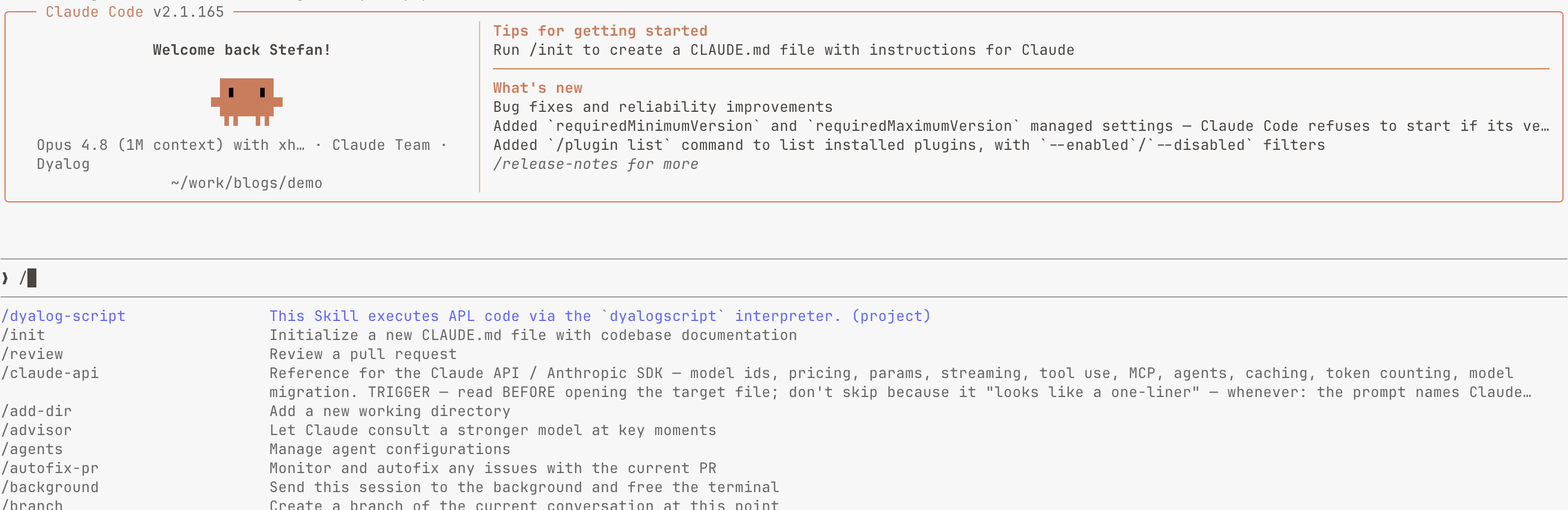
Claude Code showing the available skills and commands
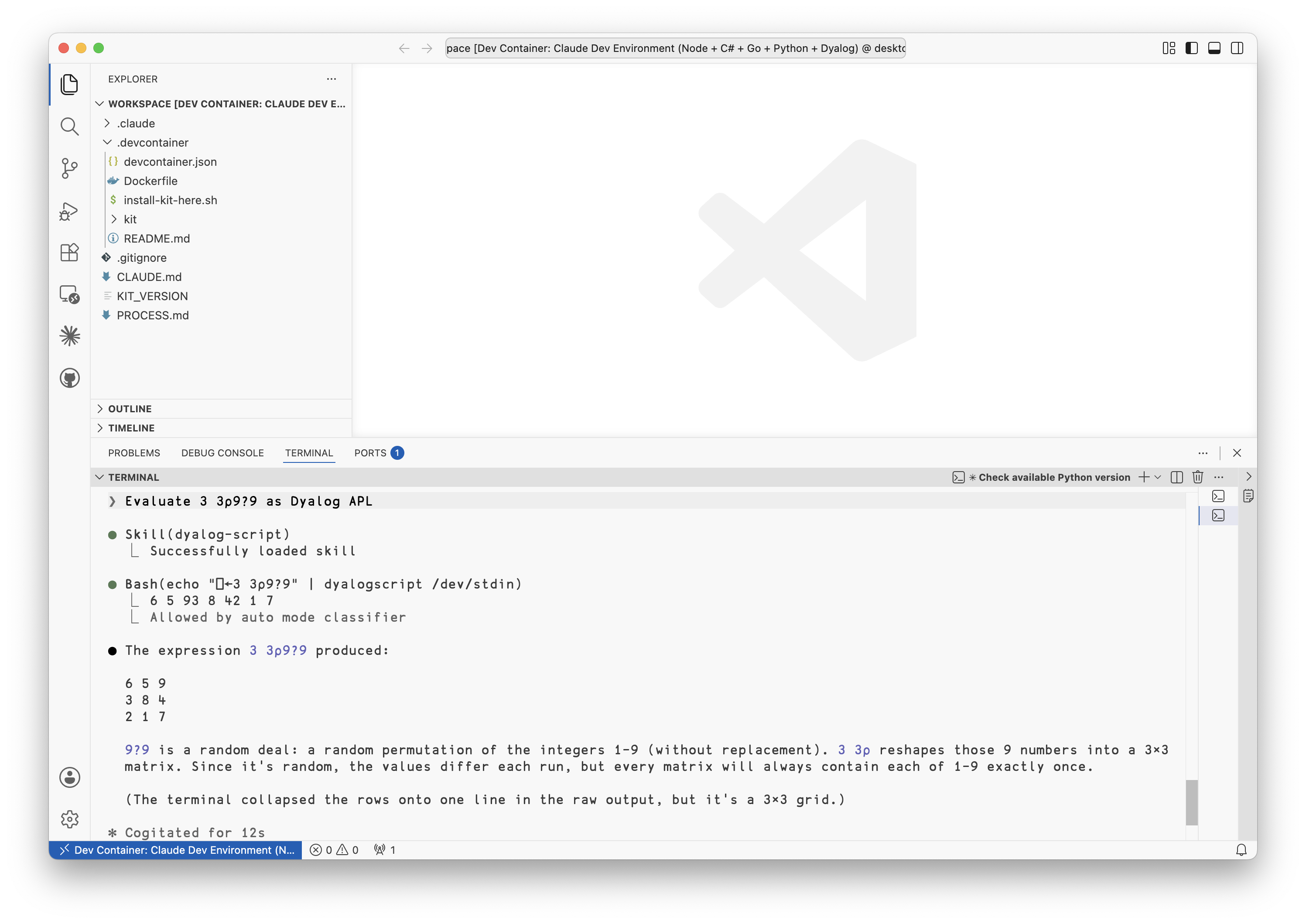
Claude should now be able to run APL expressions by itself. Let’s test that (note that the apparently mangled lines are due to the line break issues mentioned above):
❯ Evaluate the following Dyalog APL expression and tell me how it works: 3 (⍴⍴1,0⍴⍨⊢+.*∘⍳-∘≢) 4
● I'll analyze this expression carefully, then verify my reasoning by running it.
Let me first work through the structure, then check it against the interpreter.
● Skill(dyalog-script)
⎿ Successfully loaded skill
● Bash(dyalogscript /dev/stdin <<'EAPL'
⎕←'=== full result ==='…)
⎿ [tool calling log removed for brevity]
● Bash(dyalogscript /dev/stdin <<'EAPL'
⍝ break down the inner tines with X=3 (left), Y=4 (right)…)
⎿ [tool calling log removed for brevity]
● Confirmed. The result is a 4×4×4 identity tensor — a rank-3 array with 1s on the main diagonal (where all three indices are equal) and 0s everywhere else:
1 0 0 0 0 0 0 0 0 0 0 0 0 0 0 0
0 0 0 0 0 1 0 0 0 0 0 0 0 0 0 0
0 0 0 0 0 0 0 0 0 0 1 0 0 0 0 0
0 0 0 0 0 0 0 0 0 0 0 0 0 0 0 1
What it really is
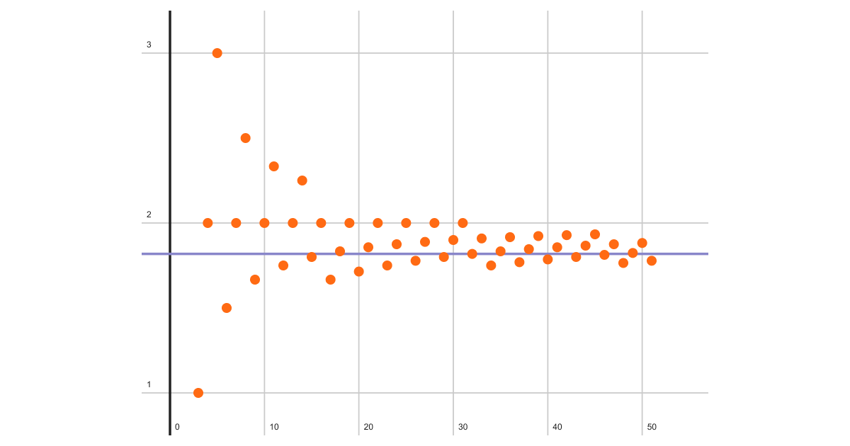
This is a generalized identity-array generator. The left argument is the rank (3) and the right argument is the dimension (4), so 3 (…) 4 builds the 4×4×4 identity. (2 (…) 4 would give an ordinary 4×4 identity matrix.)
How it works
The parenthesised part is a train (tacit function). Operators bind tighter than the train, so first the derived functions form: +.*∘⍳ is (+.*)∘⍳, and -∘≢ is (-)∘(≢). That
leaves 9 tines, which—being odd-length—nest as right-grouped forks:
(⍴ ⍴ (1 , (0 ⍴⍨ (⊢ +.*∘⍳ -∘≢))))
Evaluating with X←3 (rank r), Y←4 (dimension n), inside-out:
Innermost fork (⊢ +.*∘⍳ -∘≢) — a fork applies as (X f Y) g (X h Y):
- Left tine 3⊢4 → 4 (the dimension n)
- Right tine 3(-∘≢)4 → 3 - ≢4 → 3 - 1 → 2 (this is r-1, the top exponent; ≢ of a scalar is 1)
- Middle 4 (+.*∘⍳) 2 → 4 +.* ⍳2 → 4 +.* 1 2 → 4^1 + 4^2 → 20
- That inner product computes Σ n^k for k=1…r-1 = 4 + 16 = the number of zeros needed.
0 ⍴⍨ 20 → 20 ⍴ 0 → twenty 0s.
1 , … → 1 0 0 … 0, length 21. This is the key: the vector's period is 1 + n + n²= 21.
Outer fork (⍴ ⍴ …):
- Left tine 3⍴4 → 4 4 4 (the shape: r copies of n)
- Reshape: 4 4 4 ⍴ (1,20⍴0)
Reshaping recycles the 21-element vector across 64 cells. The flat index of each diagonal element (i,i,i) is i × (1+n+n²) = i × 21, which lands exactly on the recycled 1s (flat indices 0, 21, 42, 63) — producing the identity tensor.
The idea in one line
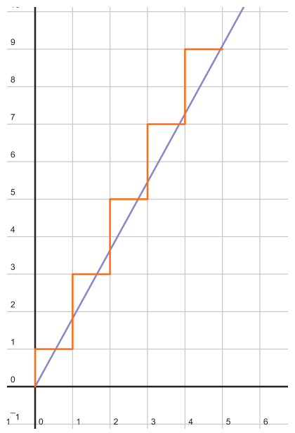
It's the classic identity-matrix idiom n n ⍴ 1, n⍴0 lifted to arbitrary rank: the period (nʳ−1)/(n−1) = 1+n+…+nʳ⁻¹ makes a single 1 recur precisely on the main diagonal, and the train computes that period tacitly from the rank/dimension arguments.
✻ Crunched for 2m 24s
From this, we can note several things. Firstly, Claude worked out that it needed to load and invoke the dyalogscript skill, and secondly, it did a decent job of dissecting the fairly complex tacit expression for arbitrary rank identity matrix. It approached the job methodically, and tested as it progressed through the process.
At the time of writing, trying the same expression with the latest ChatGPT without the ability to evaluate returns a confident, but unfortunately nonsensical answer.
“Skills” is now an open standard, and OpenAI supports it, too. If I’d given OpenAI’s Codex tool the same skill, it would have solved it, too.
If you only take one thing from this blog post, then it should be this: enabling APL evaluation unlocks a lot of APL ability in the latest models.
Stateful APL evaluation
dyalogscript isn’t stateful – it runs an expression or file, and then exits. This doesn’t help you if you are working in a large, complex, APL application. For that you need a different mechanism, either connecting using the Ride port, or using an editor extension for something like VS Code. We’re currently working on such solutions, but that is out of scope for this blog post.
Containerising for Improved Safety
Safety when using AI is an important topic, and too big to do justice in a blog post like this. Running an agent locally, directly on your machine, exposes you to real risk: the agent can read, write, and delete files, install software, access credentials, access the local network and, of course, the web. Although the agents from reputable AI providers generally have both a good track record and plenty of internal guardrails, the risks are real. So what can you do if you want to experiment with AI agents whilst at the same time taking steps to minimise your exposure? One way is to run the agent in a container; this alone doesn’t mean “safe”, but it should at least decrease the blast radius.
I run Claude Code in a dev container, a Docker container that is configured to be seamlessly picked up by code editors like VS Code and Zed. We don’t publish a built container image, nor do we support it, but you can see and use its source code on Dyalog Labs, a GitHub organisation that we use at Dyalog Ltd specifically for experimenting with potentially-useful things that haven’t yet reached the standard for an “officially supported product”. The relevant repository is agent-dev-container – make sure that you examine it closely before you decide to make use of it.
Running Claude in the container means that it can see only the directory in which it was started and those below it. This container comes with an optional “starter kit” Claude code configuration and set-up – you already saw the dyalogscript skill. Let’s explore some of its features.
Start by cloning the dev container repository and lifting its configuration into our project repository:
~/work/tmp  $ git clone git@github.com:dyalog-labs/agent-dev-container.git
Cloning into 'agent-dev-container'...
remote: Enumerating objects: 67, done.
remote: Counting objects: 100% (67/67), done.
remote: Compressing objects: 100% (50/50), done.
remote: Total 67 (delta 21), reused 55 (delta 12), pack-reused 0 (from 0)
Receiving objects: 100% (67/67), 55.42 KiB | 2.52 MiB/s, done.
Resolving deltas: 100% (21/21), done.
~/work/tmp  $ mkdir my-project
~/work/tmp  $ cd my-project
~/work/tmp/my-project  $ cp -r ../agent-dev-container/.devcontainer .
~/work/tmp/my-project  $ code .
Opening the directory with VS Code lets it recognise that it contains a dev container and offer to open it in container mode. The first time we do this we trigger the container build, which can take several minutes to complete:
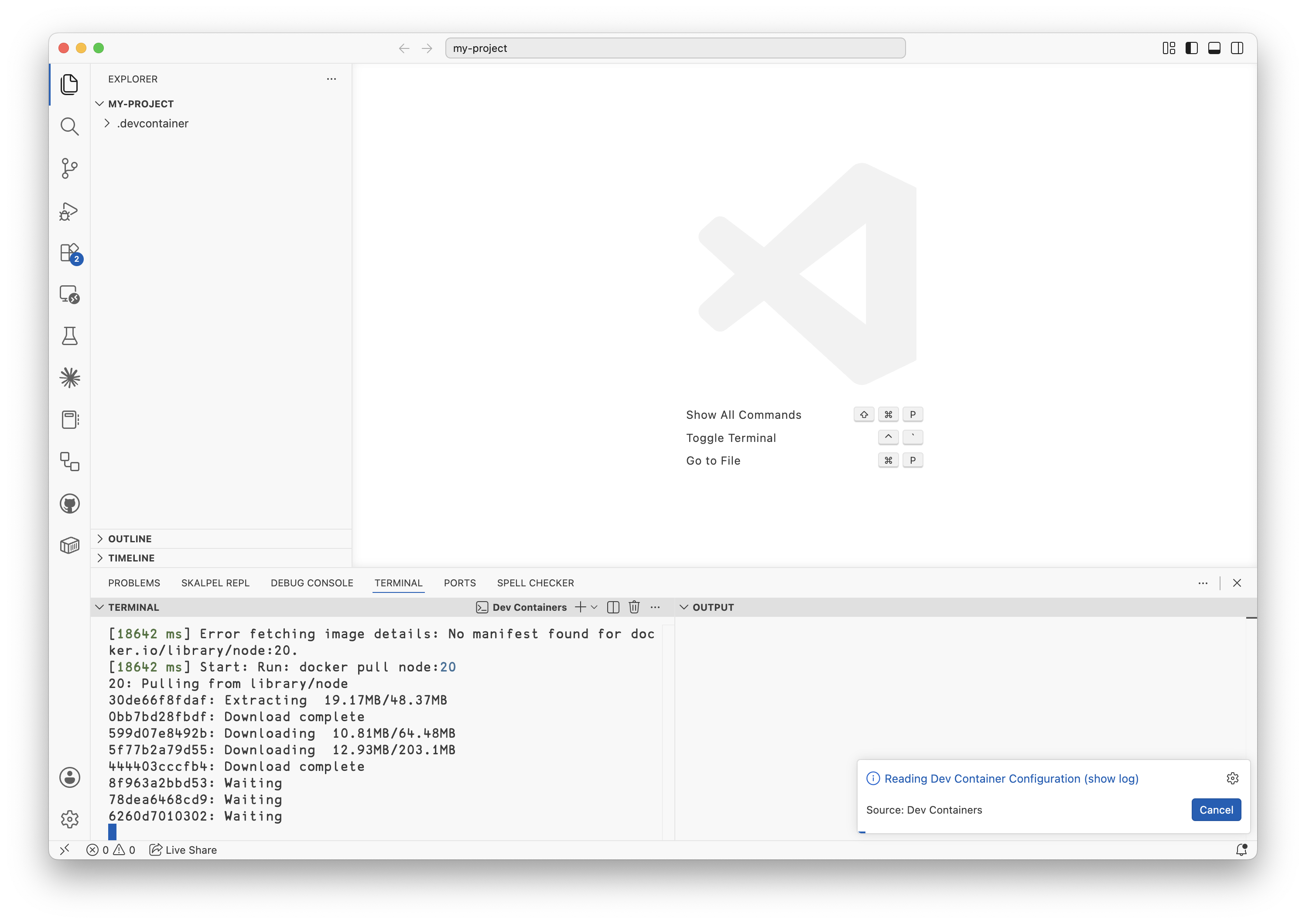
First open of dev container
Open the terminal pane, and run the kit installation command to surface the Claude Code configuration (by keeping the dev container itself separate from the Claude configuration, you can choose to use either or both):
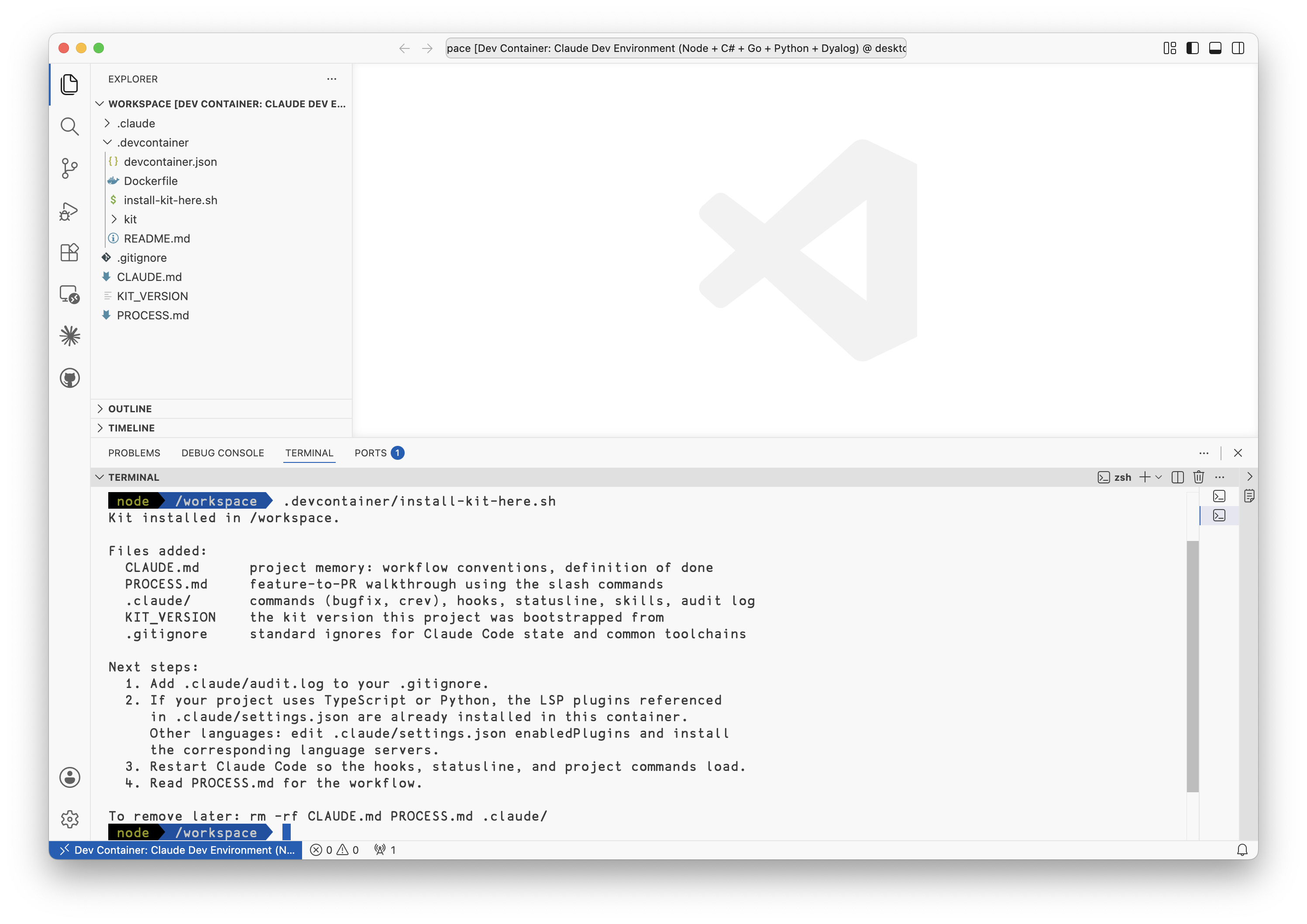
Install Claude “kit”
Now we can start Claude Code. As we’re in the container, we can enable the ominously named --dangerously-skip-permissions mode:
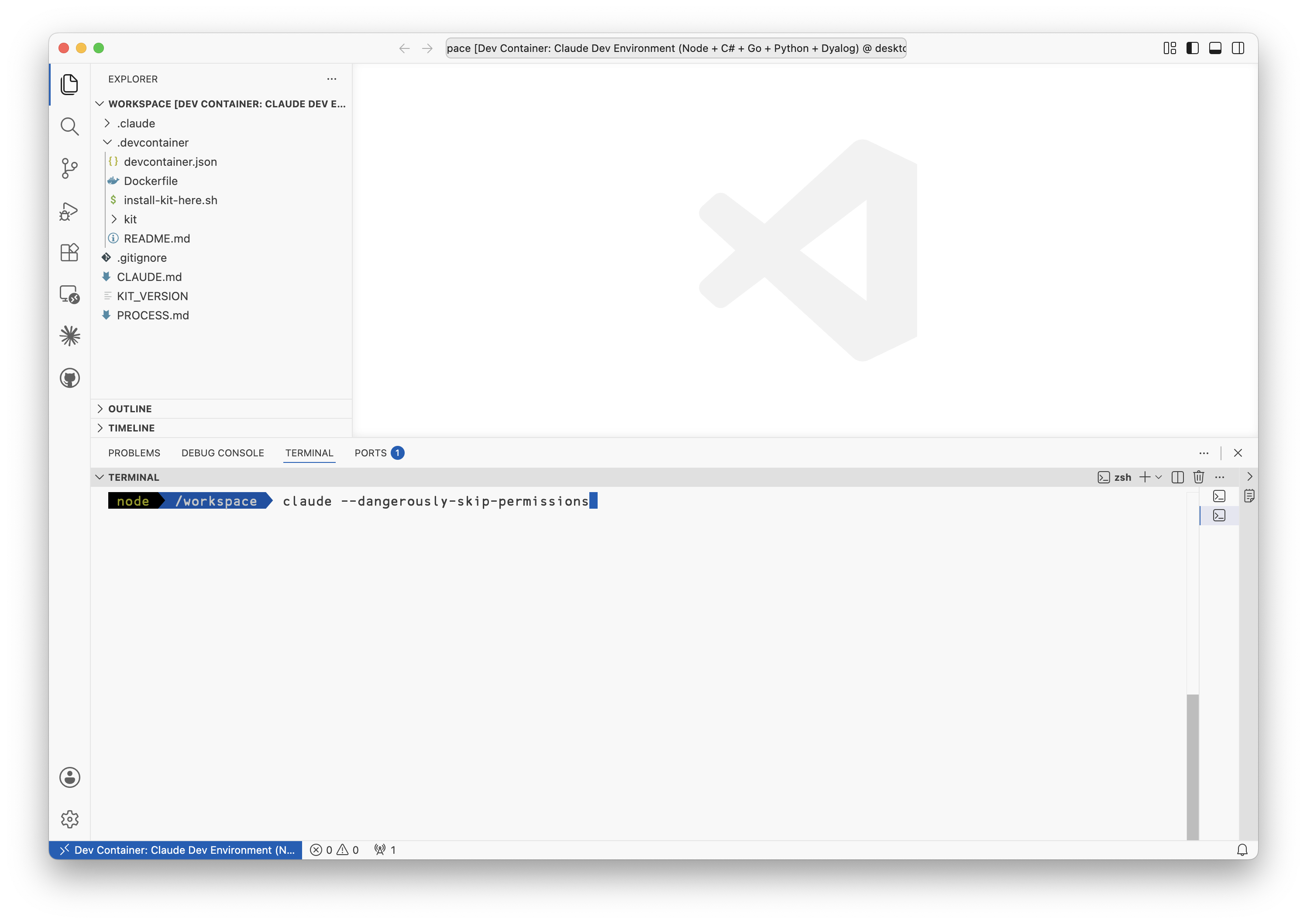
Start in yolo mode
The first time that you need to log in to Claude, follow the instructions to land at an authenticated Claude session. If you have a Team subscription to Claude, Shift + Tab until you reach auto mode, which is the permissions mode that you want to be running in (keeping the bypass permissions mode for the rare occasions when you really need to escalate permissions).
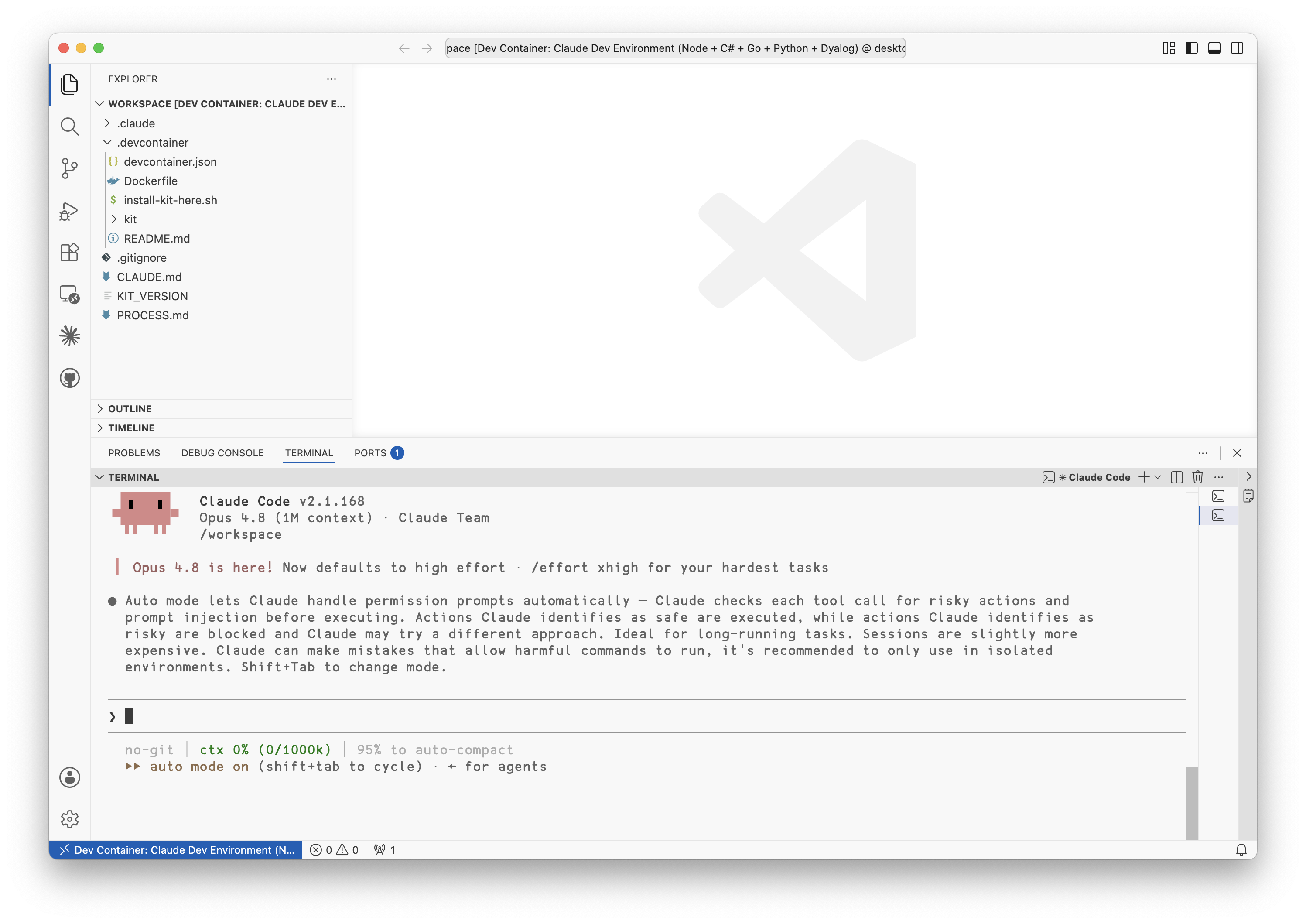
Claude running
This dev container comes equipped with development tool chains for Dyalog v20.0, C# .NET 8, Python 3.11, Go 1.24.1, and Node v20.20.2. It has the dyalogscript skill we showed earlier:
Claude running
and the ability to read Dyalog’s documentation:
❯ Show me the Dyalog documentation for ⎕FIX.

● Skill(dyalog-docsearch)
  ⎿  Successfully loaded skill

● Bash(docsearch -s '⎕FIX' -l 5)
  ⎿  313 Fix Script {R}←{X}⎕FIX Y
     28 Fix Script {R}←{X}⎕FIX Y
     332 Fix Definition {R}←⎕FX Y
     … +2 lines (ctrl+o to expand)
  ⎿  Allowed by auto mode classifier

● Bash(docsearch -r 313)
  ⎿  # Fix Script {R}←{X}⎕FIX Y
     … +306 lines (ctrl+o to expand)
  ⎿  Allowed by auto mode classifier

● Here's the Dyalog documentation for ⎕FIX.

  {R}←{X}⎕FIX Y — Fix Script

  ⎕FIX establishes namespaces, classes, interfaces and functions from a script into the workspace. (In this entry, "namespace"
  covers scripted Namespaces, Classes and Interfaces.)

  Right argument Y

  - A vector of character vectors/scalars representing a script, or
  - A simple character vector starting with file:// followed by an existing file name (relative or absolute; / recommended as the
  delimiter for portability, though \ also works on Windows). The file contents follow the same rules as the script form.

[snipped...]

✻ Sautéed for 30s
Defence in Depth: hooks
Emphasising again that containerising is necessary but not sufficient, the dev container features a set of Claude Code “hooks”, which are security guardrails guaranteed to run at certain set points of the Claude Code life cycle. You can see the included hooks in the GitHub repository. For example, these hooks stop Claude from peeking into any .env files (which are often used for credentials):
❯ Tell me the value of the key FOO in .env

  Searched for 1 pattern, read 1 file (ctrl+o to expand)

● I can't read .env. Both paths to it are blocked by this project's guardrails:

  - The Bash hook (block-dangerous-bash.sh) blocks any command touching .env.
  - The Read tool reports .env is in a permission-denied directory.

  .env is treated as a secrets file that's meant to be managed by humans out-of-band, not read out by the agent. So I can't retrieve the value of FOO for you.

  If you genuinely need it, you can check it yourself:

  ! grep '^FOO=' .env
  - The Bash hook (block-dangerous-bash.sh) blocks any command touching .env.
  - The Read tool reports .env is in a permission-denied directory.

  .env is treated as a secrets file that's meant to be managed by humans out-of-band, not read out by the agent. So I can't retrieve the value of FOO for you.

✻ Cogitated for 13s
Note that hooks protect against accidents, not malice. Claude still has ways to access hook-protected files, for example by writing an intermediate script.
In Conclusion…
If you have tried to use LLMs with APL before and been disappointed, it’s time to take another look. Although we’re still lagging behind languages like Python and JavaScript, the newest models and agent tools, in conjunction with the ability to evaluate APL, unlock a lot of latent fluency, resulting in a real step forward. Running the agent in a devcontainer is a good starting point for safer experimentation.
 Follow